Flux across curves in a vector field Consider the vector Field F = 〈 y, x 〉 shown in the figure. a. Compute the outward flux across the quarter circle C : r (t) = 〈2 cos t , 2 sin t ), for 0 ≤ t ≤ π /2 . b. Compute the outward flux across the quarter circle C : r (t) = 〈2 cos t , 2 sin t ), for π /2 ≤ t ≤ π. c. Explain why the flux across the quarter circle in the third quadrant equals the flux computed in part (a). d. Explain why the flux across the quarter circle in the fourth quadrant equals the flux computed in part (b). e. What is the outward flux across the full circle?
Flux across curves in a vector field Consider the vector Field F = 〈 y, x 〉 shown in the figure. a. Compute the outward flux across the quarter circle C : r (t) = 〈2 cos t , 2 sin t ), for 0 ≤ t ≤ π /2 . b. Compute the outward flux across the quarter circle C : r (t) = 〈2 cos t , 2 sin t ), for π /2 ≤ t ≤ π. c. Explain why the flux across the quarter circle in the third quadrant equals the flux computed in part (a). d. Explain why the flux across the quarter circle in the fourth quadrant equals the flux computed in part (b). e. What is the outward flux across the full circle?
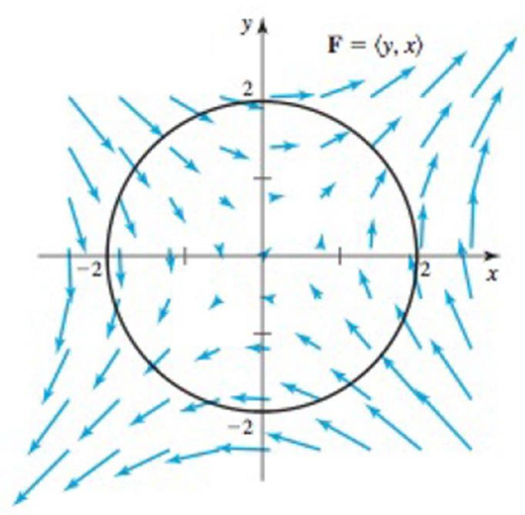
Flux across curves in a vector field Consider the vector Field F = 〈y, x〉 shown in the figure.
a. Compute the outward flux across the quarter circle C: r(t) = 〈2 cos t, 2 sin t), for 0 ≤ t ≤ π/2.
b. Compute the outward flux across the quarter circle C: r(t) = 〈2 cos t, 2 sin t), for π/2 ≤ t ≤ π.
c. Explain why the flux across the quarter circle in the third quadrant equals the flux computed in part (a).
d. Explain why the flux across the quarter circle in the fourth quadrant equals the flux computed in part (b).
e. What is the outward flux across the full circle?
Quantities that have magnitude and direction but not position. Some examples of vectors are velocity, displacement, acceleration, and force. They are sometimes called Euclidean or spatial vectors.
Given lim x-4 f (x) = 1,limx-49 (x) = 10, and lim→-4 h (x) = -7 use the limit properties
to find lim→-4
1
[2h (x) — h(x) + 7 f(x)] :
-
h(x)+7f(x)
3
O DNE
17. Suppose we know that the graph below is the graph of a solution to dy/dt = f(t).
(a) How much of the slope field can
you sketch from this information?
[Hint: Note that the differential
equation depends only on t.]
(b) What can you say about the solu-
tion with y(0) = 2? (For example,
can you sketch the graph of this so-
lution?)
y(0) = 1
y
AN
(b) Find the (instantaneous) rate of change of y at x = 5.
In the previous part, we found the average rate of change for several intervals of decreasing size starting at x = 5. The instantaneous rate of
change of fat x = 5 is the limit of the average rate of change over the interval [x, x + h] as h approaches 0. This is given by the derivative in the
following limit.
lim
h→0
-
f(x + h) − f(x)
h
The first step to find this limit is to compute f(x + h). Recall that this means replacing the input variable x with the expression x + h in the rule
defining f.
f(x + h) = (x + h)² - 5(x+ h)
=
2xh+h2_
x² + 2xh + h² 5✔
-
5
)x - 5h
Step 4
-
The second step for finding the derivative of fat x is to find the difference f(x + h) − f(x).
-
f(x + h) f(x) =
= (x²
x² + 2xh + h² -
])-
=
2x
+ h² - 5h
])x-5h) - (x² - 5x)
=
]) (2x + h - 5)
Macbook Pro
Need a deep-dive on the concept behind this application? Look no further. Learn more about this topic, calculus and related others by exploring similar questions and additional content below.
01 - What Is an Integral in Calculus? Learn Calculus Integration and how to Solve Integrals.; Author: Math and Science;https://www.youtube.com/watch?v=BHRWArTFgTs;License: Standard YouTube License, CC-BY


 Calculus: Early TranscendentalsCalculusISBN:9781285741550Author:James StewartPublisher:Cengage Learning
 Thomas' Calculus (14th Edition)CalculusISBN:9780134438986Author:Joel R. Hass, Christopher E. Heil, Maurice D. WeirPublisher:PEARSON
 Calculus: Early Transcendentals (3rd Edition)CalculusISBN:9780134763644Author:William L. Briggs, Lyle Cochran, Bernard Gillett, Eric SchulzPublisher:PEARSON
 Calculus: Early TranscendentalsCalculusISBN:9781319050740Author:Jon Rogawski, Colin Adams, Robert FranzosaPublisher:W. H. Freeman
 Calculus: Early Transcendental FunctionsCalculusISBN:9781337552516Author:Ron Larson, Bruce H. EdwardsPublisher:Cengage Learning