At a particular axial station, velocity and temperature profiles for laminar flow in a parallel plate channel have the form u ( y ) = 0.75 [ 1 − ( y / y 0 ) 2 ] T ( y ) = 5.0 + 95.66 ( y / y 0 ) 2 − 47.83 ( y / y 0 ) 4 with units of m/s and °C. respectively. Determine corresponding values of the mean velocity, u m , and mean (or hulk) temperature, T m . Plot the velocity and temperature distributions. Do your values of u m and T m appear reasonable?
At a particular axial station, velocity and temperature profiles for laminar flow in a parallel plate channel have the form u ( y ) = 0.75 [ 1 − ( y / y 0 ) 2 ] T ( y ) = 5.0 + 95.66 ( y / y 0 ) 2 − 47.83 ( y / y 0 ) 4 with units of m/s and °C. respectively. Determine corresponding values of the mean velocity, u m , and mean (or hulk) temperature, T m . Plot the velocity and temperature distributions. Do your values of u m and T m appear reasonable?
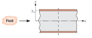
At a particular axial station, velocity and temperature profiles for laminar flow in a parallel plate channel have the form
u
(
y
)
=
0.75
[
1
−
(
y
/
y
0
)
2
]
T
(
y
)
=
5.0
+
95.66
(
y
/
y
0
)
2
−
47.83
(
y
/
y
0
)
4
with units of m/s and °C. respectively.
Determine corresponding values of the mean velocity,
u
m
, and mean (or hulk) temperature,
T
m
. Plot the velocity and temperature distributions. Do your values of
u
m
and
T
m
appear reasonable?
(I) [40 Points] Using centered finite difference approximations as done in class, solve the equation for O:
d20
dx²
+ 0.010+ Q=0
subject to the boundary conditions shown in the stencil below. Do this for two values of Q: (a) Q = 0.3,
and (b) Q= √(0.5 + 2x)e-sinx (cos(5x)+x-0.5√1.006-x| + e −43*|1+.001+x* | * sin (1.5 − x) +
(cosx+0.001 + ex-1250+ sin (1-0.9x)|) * x - 4.68x4. For Case (a) (that is, Q = 0.3), use the stencil in Fig.
1. For Case (b), calculate with both the stencils in Fig. 1 and Fig 2. For all the three cases, show a table as
well as a plot of O versus x. Discuss your results. Use MATLAB and hand in the MATLAB codes.
1
0=0
x=0
2
3
4
0=1
x=1
Fig 1
1 2 3 4 5 6 7 8 9 10
11
0=0
x=0
0=1
x=1
Fig 2
Fig 2
(II) [60 Points] Using centered finite difference approximation as done in class, solve the equation:
020 020
+
მx2 მy2
+0.0150+Q=0
subject to the boundary conditions shown in the stencils below. Do this for two values of Q: (a) Q = 0.3,
and (b) Q = 10.5x² + 1.26 * 1.5 x 0.002 0.008. For Case (a) (that is, Q = 0.3) use Fig 3. For Case (b),
use both Fig. 3 and Fig 4. For all the three cases, show a table as well as the contour plots of versus
(x, y), and the (x, y) heat flux values at all the nodes on the boundaries x = 1 and y = 1. Discuss your
results. Use MATLAB and hand in the MATLAB codes. (Note that the domain is (x, y)e[0,1] x [0,1].)
0=0
0=0
4
8
12
16
10
Ꮎ0
15
25
9
14
19
24
3
11
15
0=0
8-0
0=0
3
8
13
18
23
2
6
сл
5
0=0
10
14
6
12
17
22
1
6
11
16
21
13
e=0
Fig 3
Fig 4
Textbook: Numerical Methods for Engineers, Steven C. Chapra and Raymond P. Canale, McGraw-Hill, Eighth
Edition (2021).
Ship construction question. Sketch and describe the forward arrangements of a ship. Include componets of the structure and a explanation of each part/ term.
Ive attached a general fore end arrangement. Simplfy construction and give a brief describion of the terms.
Need a deep-dive on the concept behind this application? Look no further. Learn more about this topic, mechanical-engineering and related others by exploring similar questions and additional content below.


 Elements Of ElectromagneticsMechanical EngineeringISBN:9780190698614Author:Sadiku, Matthew N. O.Publisher:Oxford University Press
 Mechanics of Materials (10th Edition)Mechanical EngineeringISBN:9780134319650Author:Russell C. HibbelerPublisher:PEARSON
 Thermodynamics: An Engineering ApproachMechanical EngineeringISBN:9781259822674Author:Yunus A. Cengel Dr., Michael A. BolesPublisher:McGraw-Hill Education
 Control Systems EngineeringMechanical EngineeringISBN:9781118170519Author:Norman S. NisePublisher:WILEY
 Mechanics of Materials (MindTap Course List)Mechanical EngineeringISBN:9781337093347Author:Barry J. Goodno, James M. GerePublisher:Cengage Learning
 Engineering Mechanics: StaticsMechanical EngineeringISBN:9781118807330Author:James L. Meriam, L. G. Kraige, J. N. BoltonPublisher:WILEY