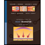
Introduction to Heat Transfer
6th Edition
ISBN: 9780470501962
Author: Frank P. Incropera, David P. DeWitt, Theodore L. Bergman, Adrienne S. Lavine
Publisher: Wiley, John & Sons, Incorporated
expand_more
expand_more
format_list_bulleted
Question
Chapter 2, Problem 2.20P
(a)
To determine
The differential equation that could be solved for the temperature of the metal versus time.
(b)
To determine
The unknown metal by comparing measured and predicted thermal responses.
Expert Solution & Answer
Want to see the full answer?
Check out a sample textbook solution
Students have asked these similar questions
Auto Controls
Design a PID controller for thefollowing system so that the modified system satisfies the followingspecifications : 1. settling time ,ts = 1.96 s and % Overshoot Mp = 70.7 %
Assume a non-dominant pole at s = -15 to solve the problem
The plot the compensated andThen plot the uncompensated system in MATLAB.
what can you see from the plot ? what is your observation ?
Fourth year
Monthly exam\3
2024-2025
Power plant
Time: 1 Hr
Q1. A gas turbine power plant operates on a modified Brayton cycle consisting
of two-stage compression with intercooling to the initial temperature
between stages, two-stage expansion with reheating to the maximum cycle
temperature, and two regenerative heat exchangers.
The following data is given:
Inlet air temperature: 300 K
Maximum cycle temperature: 1400 K
Pressure ratio across each compressor stage: 4
Pressure ratio across each turbine stage: 4
Isentropic efficiency of compressors and turbines: 85%
Effectiveness of each regenerator: 80%
a) Draw a schematic and T-s diagram of the cycle.
b) Determine the thermal efficiency of the cycle.
c) Calculate the net specific work output (in kJ/kg).
d) Discuss the impact of regenerators on the cycle performance.
Examiner
Prof. Dr. Adil Al-Kumait
Auto Controls
The figure is a schematic diagram of an aircraft elevator control system. The input to the systemin the deflection angle of the control lever , and the output is the elevator angle phi.show that for each angle theta of the control lever ,there is a corresponding elevator angle phi.
Then find Y(s)/theta(s) and simplify the resulting transfer function . Also note from the diagram that y and phi is related
Chapter 2 Solutions
Introduction to Heat Transfer
Ch. 2 - Assume steady-state, one-dimensional heat...Ch. 2 - Assume steady-state, one-dimensional conduction in...Ch. 2 - A hot water pipe with outside radius r1 has a...Ch. 2 - A spherical shell with inner radius r1 and outer...Ch. 2 - Assume steady-state, one-dimensional heat...Ch. 2 - A composite rod consists of two different...Ch. 2 - A solid, truncated cone serves as a support for a...Ch. 2 - To determine the effect of the temperature...Ch. 2 - Prob. 2.9PCh. 2 - A one-dimensional plane wall of thickness 2L=100mm...
Ch. 2 - Consider steady-state conditions for...Ch. 2 - Consider a plane wall 100 mm thick and of thermal...Ch. 2 - Prob. 2.13PCh. 2 - In the two-dimensional body illustrated, the...Ch. 2 - Consider the geometry of Problem 2.14 for the case...Ch. 2 - Steady-state, one-dimensional conduction occurs in...Ch. 2 - Prob. 2.17PCh. 2 - Prob. 2.18PCh. 2 - Consider a 300mm300mm window in an aircraft. For a...Ch. 2 - Prob. 2.20PCh. 2 - Use IHT to perform the following tasks. Graph the...Ch. 2 - Calculate the thermal conductivity of air,...Ch. 2 - A method for determining the thermal conductivity...Ch. 2 - Prob. 2.24PCh. 2 - Prob. 2.25PCh. 2 - At a given instant of time, the temperature...Ch. 2 - Prob. 2.27PCh. 2 - Uniform internal heat generation at q.=5107W/m3 is...Ch. 2 - Prob. 2.29PCh. 2 - The steady-state temperature distribution in a...Ch. 2 - The temperature distribution across a wall 0.3 m...Ch. 2 - Prob. 2.32PCh. 2 - Prob. 2.33PCh. 2 - Prob. 2.34PCh. 2 - Prob. 2.35PCh. 2 - Prob. 2.36PCh. 2 - Prob. 2.37PCh. 2 - One-dimensional, steady-state conduction with no...Ch. 2 - One-dimensional, steady-state conduction with no...Ch. 2 - The steady-state temperature distribution in a...Ch. 2 - One-dimensional, steady-state conduction with no...Ch. 2 - Prob. 2.42PCh. 2 - Prob. 2.43PCh. 2 - Prob. 2.44PCh. 2 - Beginning with a differential control volume in...Ch. 2 - A steam pipe is wrapped with insulation of inner...Ch. 2 - Prob. 2.47PCh. 2 - Prob. 2.48PCh. 2 - Two-dimensional, steady-state conduction occurs in...Ch. 2 - Prob. 2.50PCh. 2 - Prob. 2.51PCh. 2 - A chemically reacting mixture is stored in a...Ch. 2 - A thin electrical heater dissipating 4000W/m2 is...Ch. 2 - The one-dimensional system of mass M with constant...Ch. 2 - Consider a one-dimensional plane wall of thickness...Ch. 2 - A large plate of thickness 2L is at a uniform...Ch. 2 - Prob. 2.57PCh. 2 - Prob. 2.58PCh. 2 - A plane wall has constant properties, no internal...Ch. 2 - A plane wall with constant properties is initially...Ch. 2 - Consider the conditions associated with Problem...Ch. 2 - Prob. 2.62PCh. 2 - A spherical particle of radius r1 experiences...Ch. 2 - Prob. 2.64PCh. 2 - A plane wall of thickness L=0.1m experiences...Ch. 2 - Prob. 2.66PCh. 2 - A composite one-dimensional plane wall is of...Ch. 2 - Prob. 2.68PCh. 2 - The steady-state temperature distribution in a...
Knowledge Booster
Learn more about
Need a deep-dive on the concept behind this application? Look no further. Learn more about this topic, mechanical-engineering and related others by exploring similar questions and additional content below.Similar questions
- Liquid hexane flows through a counter flow heat exchanger at 5 m3/h as shown in Figure E5.5.The hexane enters the heat exchanger at 90°C. Water, flowing at 5 m3/h, is used to cool the hexane.The water enters the heat exchanger at 15°C. The UA product of the heat exchanger is found to be2.7 kW/K. Determine the outlet temperatures of the hot and cold fluids and the heat transfer ratebetween them using LMTD method.arrow_forwardDetermine the fluid outlet temperatures and the heat transfer rate for the counter flow heatexchanger described in Problem 3 using the ε-NTU model. Assume that the properties can beevaluated at the given fluid inlet temperatures.arrow_forwardSection View - practice Homework 0.5000 3.0000 2,0000 1.0000arrow_forward
- Drawing the section view for the following multiview drawing AutoCAD you see the section pratice I need to show how to autocadarrow_forwardA boiler with 80% efficiency produces steam at 40bar and 500 C at a rate of 1.128kg/s. The temperature of the feed water is raised from 25 C to 125 C in the economizer and the ambient air is drawn to the boiler at a rate of 2.70 kg/s at 16 C. The flue gases leave the chimney at rate of 3 kg/s at 150 C with specific heat of 1.01 kJ/kg.K. The dryness fraction of steam collected in the steam drum is 0.95. 1- Determine the heat value of the fuel. 2- The equivalence evaporation. 3- Draw the heat balance sheet.arrow_forwardA rotating shaft is made of 42 mm by 4 mm thick cold-drawn round steel tubing and has a 6 mm diameter hole drilled transversely through it. The shaft is subjected to a pulsating torque fluctuating from 20 to 160 Nm and a completely reversed bending moment of 200 Nm. The steel tubing has a minimum strength of Sut = 410 MPa (60 ksi). The static stress-concentration factor for the hole is 2.4 for bending and 1.9 for torsion. The maximum operating temperature is 400˚C and a reliability of 99.9% is to be assumed. Find the factor of safety for infinite life using the modified Goodman failure criterion.arrow_forward
- I need help with a MATLAB code. This code just keeps running and does not give me any plots. I even reduced the tolerance from 1e-9 to 1e-6. Can you help me fix this? Please make sure your solution runs. % Initial Conditions rev = 0:0.001:2; g1 = deg2rad(1); g2 = deg2rad(3); g3 = deg2rad(6); g4 = deg2rad(30); g0 = deg2rad(0); Z0 = 0; w0 = [0; Z0*cos(g0); -Z0*sin(g0)]; Z1 = 5; w1 = [0; Z1*cos(g1); -Z1*sin(g1)]; Z2 = 11; w2 = [0; Z2*cos(g2); -Z2*sin(g2)]; [v3, psi3, eta3] = Nut_angle(Z2, g2, w2); plot(v3, psi3) function dwedt = K_DDE(~, w_en) % Extracting the initial condtions to a variable % Extracting the initial condtions to a variable w = w_en(1:3); e = w_en(4:7); Z = w_en(8); I = 0.060214; J = 0.015707; x = (J/I) - 1; y = Z - 1; s = Z; % Kinematic Differential Equations dedt = zeros(4,1); dedt(1) = pi*(e(3)*(s-w(2)-1) + e(2)*w(3) + e(4)*w(1)); dedt(2) = pi*(e(4)*(w(2)-1-s) + e(3)*w(1) - e(1)*w(3)); dedt(3) = pi*(-e(1)*(s-w(2)-1) - e(2)*w(1) + e(4)*w(3));…arrow_forwardalpha 1 is not zero alpha 1 can equal alpha 2 use velocity triangle to solve for alpha 1 USE MATLAB ONLY provide typed code solve for velocity triangle and dont provide copied answer Turbomachienery . GIven: vx = 185 m/s, flow angle = 60 degrees, (leaving a stator in axial flow) R = 0.5, U = 150 m/s, b2 = -a3, a2 = -b3 Find: velocity triangle , a. magnitude of abs vel leaving rotor (m/s) b. flow absolute angles (a1, a2, a3) 3. flow rel angles (b2, b3) d. specific work done e. use code to draw vel. diagram Use this code for plot % plots Velocity Tri. in Ch4 function plotveltri(al1,al2,al3,b2,b3) S1L = [0 1]; V1x = [0 0]; V1s = [0 1*tand(al3)]; S2L = [2 3]; V2x = [0 0]; V2s = [0 1*tand(al2)]; W2s = [0 1*tand(b2)]; U2x = [3 3]; U2y = [1*tand(b2) 1*tand(al2)]; S3L = [4 5]; V3x = [0 0]; V3r = [0 1*tand(al3)]; W3r = [0 1*tand(b3)]; U3x = [5 5]; U3y = [1*tand(b3) 1*tand(al3)]; plot(S1L,V1x,'k',S1L,V1s,'r',... S2L,V2x,'k',S2L,V2s,'r',S2L,W2s,'b',U2x,U2y,'g',...…arrow_forward3. Find a basis of eigenvectors and diagonalize. 4 0 -19 7 a. b. 1-42 16 12-20 [21-61arrow_forward
- 2. Find the eigenvalues. Find the corresponding eigenvectors. 6 2 -21 [0 -3 1 3 31 a. 2 5 0 b. 3 0 -6 C. 1 1 0 -2 0 7 L6 6 0 1 1 2. (Hint: λ = = 3)arrow_forwardUSE MATLAB ONLY provide typed code solve for velocity triangle and dont provide copied answer Turbomachienery . GIven: vx = 185 m/s, flow angle = 60 degrees, (leaving a stator in axial flow) R = 0.5, U = 150 m/s, b2 = -a3, a2 = -b3 Find: velocity triangle , a. magnitude of abs vel leaving rotor (m/s) b. flow absolute angles (a1, a2, a3) 3. flow rel angles (b2, b3) d. specific work done e. use code to draw vel. diagram Use this code for plot % plots Velocity Tri. in Ch4 function plotveltri(al1,al2,al3,b2,b3) S1L = [0 1]; V1x = [0 0]; V1s = [0 1*tand(al3)]; S2L = [2 3]; V2x = [0 0]; V2s = [0 1*tand(al2)]; W2s = [0 1*tand(b2)]; U2x = [3 3]; U2y = [1*tand(b2) 1*tand(al2)]; S3L = [4 5]; V3x = [0 0]; V3r = [0 1*tand(al3)]; W3r = [0 1*tand(b3)]; U3x = [5 5]; U3y = [1*tand(b3) 1*tand(al3)]; plot(S1L,V1x,'k',S1L,V1s,'r',... S2L,V2x,'k',S2L,V2s,'r',S2L,W2s,'b',U2x,U2y,'g',... S3L,V3x,'k',S3L,V3r,'r',S3L,W3r,'b',U3x,U3y,'g',...... 'LineWidth',2,'MarkerSize',10),...…arrow_forwardUSE MATLAB ONLY provide typed code solve for velocity triangle and dont provide copied answer Turbomachienery . GIven: vx = 185 m/s, flow angle = 60 degrees, R = 0.5, U = 150 m/s, b2 = -a3, a2 = -b3 Find: velocity triangle , a. magnitude of abs vel leaving rotor (m/s) b. flow absolute angles (a1, a2, a3) 3. flow rel angles (b2, b3) d. specific work done e. use code to draw vel. diagram Use this code for plot % plots Velocity Tri. in Ch4 function plotveltri(al1,al2,al3,b2,b3) S1L = [0 1]; V1x = [0 0]; V1s = [0 1*tand(al3)]; S2L = [2 3]; V2x = [0 0]; V2s = [0 1*tand(al2)]; W2s = [0 1*tand(b2)]; U2x = [3 3]; U2y = [1*tand(b2) 1*tand(al2)]; S3L = [4 5]; V3x = [0 0]; V3r = [0 1*tand(al3)]; W3r = [0 1*tand(b3)]; U3x = [5 5]; U3y = [1*tand(b3) 1*tand(al3)]; plot(S1L,V1x,'k',S1L,V1s,'r',... S2L,V2x,'k',S2L,V2s,'r',S2L,W2s,'b',U2x,U2y,'g',... S3L,V3x,'k',S3L,V3r,'r',S3L,W3r,'b',U3x,U3y,'g',...... 'LineWidth',2,'MarkerSize',10),... axis([-1 6 -4 4]), ...…arrow_forward
arrow_back_ios
SEE MORE QUESTIONS
arrow_forward_ios
Recommended textbooks for you
 Principles of Heat Transfer (Activate Learning wi...Mechanical EngineeringISBN:9781305387102Author:Kreith, Frank; Manglik, Raj M.Publisher:Cengage Learning

Principles of Heat Transfer (Activate Learning wi...
Mechanical Engineering
ISBN:9781305387102
Author:Kreith, Frank; Manglik, Raj M.
Publisher:Cengage Learning
Power Plant Explained | Working Principles; Author: RealPars;https://www.youtube.com/watch?v=HGVDu1z5YQ8;License: Standard YouTube License, CC-BY