
Videos
a.
To know that do students who graduate from high school earn more money than students who do not and will it be appropriate to use frequency histograms instead of relative frequency histograms in this setting.
a.
Answer to Problem 75E
No. it would not be appropriate to use frequency histograms instead of relative frequency histograms.
Explanation of Solution
Given a random sample of 371 U.S. residents aged 18 and older. The educational level and total personal income of each person were recorded. The data for the 57 non-graduates (No) and the 314 graduates (Yes) are displayed in the relative frequency histograms provided below:
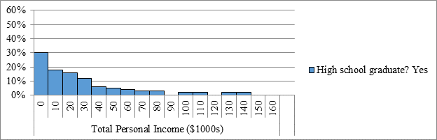
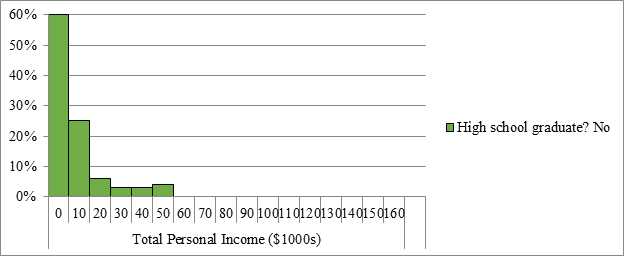
It would not be appropriate to use frequency histograms instead of relative frequency histograms, because the two histograms do not use the same number of data values (as there are 314 graduates but only 57 non-graduates). Since these two histograms would then not be based on the same number of data values, we would not be able to compare the frequency histograms.
b.
To know that do students who graduate from high school earn more money than students who do not and to compare the distributions of total personal income for these two groups.
b.
Answer to Problem 75E
Both distributions are skewed to the right.
The distribution of the nongraduates do not appear to contain any outliers, while the distribution of the graduates contains possible outliers.
The center of both distributions appears to be roughly between 0 and 10 thousand dollars.
The spread of the graduate distributions is greater than the spread for the nongraduate distribution.
Explanation of Solution
Given a random sample of 371 U.S. residents aged 18 and older. The educational level and total personal income of each person were recorded. The data for the 57 non-graduates (No) and the 314 graduates (Yes) are displayed in the relative frequency histograms provided below:
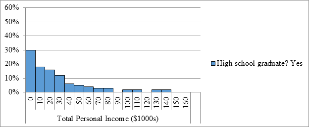
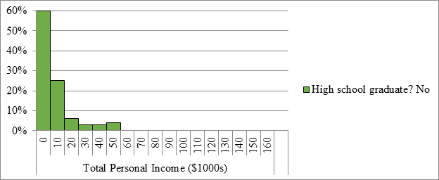
Both distributions are skewed to the right, because the highest bars are to the left in the histograms with a tail of smaller bars to the right as shown in the histograms above.
The distribution of the nongraduates do not appear to contain any outliers, because there are no gaps in the histogram. The distribution of the graduates contains possible outliers, because there are 4 bars in the histogram that are separated from the rest of the bars in the histogram with a gap.
The center of both distributions appears to be roughly between 0 and 10 thousand dollars, as we expect the center to be roughly at the highest bar in the histogram.The spread of the graduate distributions is greater than the spread for the nongraduate distribution, because the histogram for the graduates is wider compared to the histogram of the nongraduates.
Chapter 1 Solutions
PRACTICE OF STATISTICS F/AP EXAM
Additional Math Textbook Solutions
Elementary Statistics
Basic Business Statistics, Student Value Edition
Thinking Mathematically (6th Edition)
Intro Stats, Books a la Carte Edition (5th Edition)
Algebra and Trigonometry (6th Edition)


- Find the critical value for a left-tailed test using the F distribution with a 0.025, degrees of freedom in the numerator=12, and degrees of freedom in the denominator = 50. A portion of the table of critical values of the F-distribution is provided. Click the icon to view the partial table of critical values of the F-distribution. What is the critical value? (Round to two decimal places as needed.)arrow_forwardA retail store manager claims that the average daily sales of the store are $1,500. You aim to test whether the actual average daily sales differ significantly from this claimed value. You can provide your answer by inserting a text box and the answer must include: Null hypothesis, Alternative hypothesis, Show answer (output table/summary table), and Conclusion based on the P value. Showing the calculation is a must. If calculation is missing,so please provide a step by step on the answers Numerical answers in the yellow cellsarrow_forwardShow all workarrow_forward
- Show all workarrow_forwardplease find the answers for the yellows boxes using the information and the picture belowarrow_forwardA marketing agency wants to determine whether different advertising platforms generate significantly different levels of customer engagement. The agency measures the average number of daily clicks on ads for three platforms: Social Media, Search Engines, and Email Campaigns. The agency collects data on daily clicks for each platform over a 10-day period and wants to test whether there is a statistically significant difference in the mean number of daily clicks among these platforms. Conduct ANOVA test. You can provide your answer by inserting a text box and the answer must include: also please provide a step by on getting the answers in excel Null hypothesis, Alternative hypothesis, Show answer (output table/summary table), and Conclusion based on the P value.arrow_forward
 MATLAB: An Introduction with ApplicationsStatisticsISBN:9781119256830Author:Amos GilatPublisher:John Wiley & Sons Inc
 Probability and Statistics for Engineering and th...StatisticsISBN:9781305251809Author:Jay L. DevorePublisher:Cengage Learning
 Statistics for The Behavioral Sciences (MindTap C...StatisticsISBN:9781305504912Author:Frederick J Gravetter, Larry B. WallnauPublisher:Cengage Learning
 Elementary Statistics: Picturing the World (7th E...StatisticsISBN:9780134683416Author:Ron Larson, Betsy FarberPublisher:PEARSON
 The Basic Practice of StatisticsStatisticsISBN:9781319042578Author:David S. Moore, William I. Notz, Michael A. FlignerPublisher:W. H. Freeman
 Introduction to the Practice of StatisticsStatisticsISBN:9781319013387Author:David S. Moore, George P. McCabe, Bruce A. CraigPublisher:W. H. Freeman