
PRACTICE OF STATISTICS F/AP EXAM
6th Edition
ISBN: 9781319113339
Author: Starnes
Publisher: MAC HIGHER
expand_more
expand_more
format_list_bulleted
Concept explainers
Videos
Question
Chapter 1, Problem T1.10SPT
To determine
To find: the following is not a correct statement about the results of this experiment.
Expert Solution & Answer
Answer to Problem T1.10SPT
Some of the results for the low concentration of weed killer show a smaller percentage of weeds growing than some of the results for the high concentrations.
Explanation of Solution
Given:
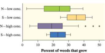
- Correct, the reason is that the in the box plot S is lying to the right comparing to the N which is indicating that the new chemical outcomes in better weed control comparing the standard weed killer.
- Correct, for both the S and N, the boxes of the box plots of higher concentrations lying to the left of the boxes of the box plots of lower concentrations, which means that more weeds grew for the low concentrations.
- Correct, the reason is that box plot of N is wider than S which is indicating that the outcomes for the standard weed killer are less variable comparing to the outcomes of the new chemical.
- Not correct, because for both S and N the boxes of the box plots of higher concentrations are lying to the left of the boxes of the box plots of lower concentrations, which means that more weeds grew for the low concentrations.
- Correct, because it is not the lowest percent of weeds for the low concentration is near 3% and the highest percent of weeds for the high concentration is near 50%, which is showing that it is possible for the low concentration to have a smaller percentage of weeds compared to the high concentration.
Hence, the correct option is (d)
Chapter 1 Solutions
PRACTICE OF STATISTICS F/AP EXAM
Ch. 1.1 - Prob. 11ECh. 1.1 - Prob. 12ECh. 1.1 - Prob. 13ECh. 1.1 - Prob. 14ECh. 1.1 - Prob. 15ECh. 1.1 - Prob. 16ECh. 1.1 - Prob. 17ECh. 1.1 - Prob. 18ECh. 1.1 - Prob. 19ECh. 1.1 - Prob. 20E
Ch. 1.1 - Prob. 21ECh. 1.1 - Prob. 22ECh. 1.1 - Prob. 23ECh. 1.1 - Prob. 24ECh. 1.1 - Prob. 25ECh. 1.1 - Prob. 26ECh. 1.1 - Prob. 27ECh. 1.1 - Prob. 28ECh. 1.1 - Prob. 29ECh. 1.1 - Prob. 30ECh. 1.1 - Prob. 31ECh. 1.1 - Prob. 32ECh. 1.1 - Prob. 33ECh. 1.1 - Prob. 34ECh. 1.1 - Prob. 35ECh. 1.1 - Prob. 36ECh. 1.1 - Prob. 37ECh. 1.1 - Prob. 38ECh. 1.1 - Prob. 39ECh. 1.1 - Prob. 40ECh. 1.1 - Prob. 41ECh. 1.1 - Prob. 42ECh. 1.1 - Prob. 43ECh. 1.1 - Prob. 44ECh. 1.2 - Prob. 45ECh. 1.2 - Prob. 46ECh. 1.2 - Prob. 47ECh. 1.2 - Prob. 48ECh. 1.2 - Prob. 49ECh. 1.2 - Prob. 50ECh. 1.2 - Prob. 51ECh. 1.2 - Prob. 52ECh. 1.2 - Prob. 53ECh. 1.2 - Prob. 54ECh. 1.2 - Prob. 55ECh. 1.2 - Prob. 56ECh. 1.2 - Prob. 57ECh. 1.2 - Prob. 58ECh. 1.2 - Prob. 59ECh. 1.2 - Prob. 60ECh. 1.2 - Prob. 61ECh. 1.2 - Prob. 62ECh. 1.2 - Prob. 63ECh. 1.2 - Prob. 64ECh. 1.2 - Prob. 65ECh. 1.2 - Prob. 66ECh. 1.2 - Prob. 67ECh. 1.2 - Prob. 68ECh. 1.2 - Prob. 69ECh. 1.2 - Prob. 70ECh. 1.2 - Prob. 71ECh. 1.2 - Prob. 72ECh. 1.2 - Prob. 73ECh. 1.2 - Prob. 74ECh. 1.2 - Prob. 75ECh. 1.2 - Prob. 76ECh. 1.2 - Prob. 77ECh. 1.2 - Prob. 78ECh. 1.2 - Prob. 79ECh. 1.2 - Prob. 80ECh. 1.2 - Prob. 81ECh. 1.2 - Prob. 82ECh. 1.2 - Prob. 83ECh. 1.2 - Prob. 84ECh. 1.2 - Prob. 85ECh. 1.2 - Prob. 86ECh. 1.3 - Prob. 87ECh. 1.3 - Prob. 88ECh. 1.3 - Prob. 89ECh. 1.3 - Prob. 90ECh. 1.3 - Prob. 91ECh. 1.3 - Prob. 92ECh. 1.3 - Prob. 93ECh. 1.3 - Prob. 94ECh. 1.3 - Prob. 95ECh. 1.3 - Prob. 96ECh. 1.3 - Prob. 97ECh. 1.3 - Prob. 98ECh. 1.3 - Prob. 99ECh. 1.3 - Prob. 100ECh. 1.3 - Prob. 101ECh. 1.3 - Prob. 102ECh. 1.3 - Prob. 103ECh. 1.3 - Prob. 104ECh. 1.3 - Prob. 105ECh. 1.3 - Prob. 106ECh. 1.3 - Prob. 107ECh. 1.3 - Prob. 108ECh. 1.3 - Prob. 109ECh. 1.3 - Prob. 110ECh. 1.3 - Prob. 111ECh. 1.3 - Prob. 112ECh. 1.3 - Prob. 113ECh. 1.3 - Prob. 114ECh. 1.3 - Prob. 115ECh. 1.3 - Prob. 116ECh. 1.3 - Prob. 117ECh. 1.3 - Prob. 118ECh. 1.3 - Prob. 119ECh. 1.3 - Prob. 120ECh. 1.3 - Prob. 121ECh. 1.3 - Prob. 122ECh. 1.3 - Prob. 123ECh. 1.3 - Prob. 124ECh. 1.3 - Prob. 125ECh. 1.3 - Prob. 126ECh. 1.3 - Prob. 127ECh. 1.3 - Prob. 128ECh. 1 - Prob. 1ECh. 1 - Prob. 2ECh. 1 - Prob. 3ECh. 1 - Prob. 4ECh. 1 - Prob. 5ECh. 1 - Prob. 6ECh. 1 - Prob. 7ECh. 1 - Prob. 8ECh. 1 - Prob. 9ECh. 1 - Prob. 10ECh. 1 - Prob. R1.1RECh. 1 - Prob. R1.2RECh. 1 - Prob. R1.3RECh. 1 - Prob. R1.4RECh. 1 - Prob. R1.5RECh. 1 - Prob. R1.6RECh. 1 - Prob. R1.7RECh. 1 - Prob. R1.8RECh. 1 - Prob. R1.9RECh. 1 - Prob. R1.10RECh. 1 - Prob. T1.1SPTCh. 1 - Prob. T1.2SPTCh. 1 - Prob. T1.3SPTCh. 1 - Prob. T1.4SPTCh. 1 - Prob. T1.5SPTCh. 1 - Prob. T1.6SPTCh. 1 - Prob. T1.7SPTCh. 1 - Prob. T1.8SPTCh. 1 - Prob. T1.9SPTCh. 1 - Prob. T1.10SPTCh. 1 - Prob. T1.11SPTCh. 1 - Prob. T1.12SPTCh. 1 - Prob. T1.13SPTCh. 1 - Prob. T1.14SPT
Additional Math Textbook Solutions
Find more solutions based on key concepts
76. Dew Point and Altitude The dew point decreases as altitude increases. If the dew point on the ground is 80°...
College Algebra with Modeling & Visualization (5th Edition)
Consider a group of 20 people. If everyone shakes hands with everyone else, how many handshakes take place?
A First Course in Probability (10th Edition)
Continuity at a point Determine whether the following functions are continuous at a. Use the continuity checkli...
Calculus: Early Transcendentals (2nd Edition)
CLT Shapes (Example 4) One of the histograms is a histogram of a sample (from a population with a skewed distri...
Introductory Statistics
Testing for a Linear Correlation. In Exercises 13-28, construct a scatterplot, and find the value of the linear...
Elementary Statistics (13th Edition)
Knowledge Booster


Learn more about
Need a deep-dive on the concept behind this application? Look no further. Learn more about this topic, statistics and related others by exploring similar questions and additional content below.Similar questions
- Harvard University California Institute of Technology Massachusetts Institute of Technology Stanford University Princeton University University of Cambridge University of Oxford University of California, Berkeley Imperial College London Yale University University of California, Los Angeles University of Chicago Johns Hopkins University Cornell University ETH Zurich University of Michigan University of Toronto Columbia University University of Pennsylvania Carnegie Mellon University University of Hong Kong University College London University of Washington Duke University Northwestern University University of Tokyo Georgia Institute of Technology Pohang University of Science and Technology University of California, Santa Barbara University of British Columbia University of North Carolina at Chapel Hill University of California, San Diego University of Illinois at Urbana-Champaign National University of Singapore McGill…arrow_forwardName Harvard University California Institute of Technology Massachusetts Institute of Technology Stanford University Princeton University University of Cambridge University of Oxford University of California, Berkeley Imperial College London Yale University University of California, Los Angeles University of Chicago Johns Hopkins University Cornell University ETH Zurich University of Michigan University of Toronto Columbia University University of Pennsylvania Carnegie Mellon University University of Hong Kong University College London University of Washington Duke University Northwestern University University of Tokyo Georgia Institute of Technology Pohang University of Science and Technology University of California, Santa Barbara University of British Columbia University of North Carolina at Chapel Hill University of California, San Diego University of Illinois at Urbana-Champaign National University of Singapore…arrow_forwardA company found that the daily sales revenue of its flagship product follows a normal distribution with a mean of $4500 and a standard deviation of $450. The company defines a "high-sales day" that is, any day with sales exceeding $4800. please provide a step by step on how to get the answers in excel Q: What percentage of days can the company expect to have "high-sales days" or sales greater than $4800? Q: What is the sales revenue threshold for the bottom 10% of days? (please note that 10% refers to the probability/area under bell curve towards the lower tail of bell curve) Provide answers in the yellow cellsarrow_forward
- Find the critical value for a left-tailed test using the F distribution with a 0.025, degrees of freedom in the numerator=12, and degrees of freedom in the denominator = 50. A portion of the table of critical values of the F-distribution is provided. Click the icon to view the partial table of critical values of the F-distribution. What is the critical value? (Round to two decimal places as needed.)arrow_forwardA retail store manager claims that the average daily sales of the store are $1,500. You aim to test whether the actual average daily sales differ significantly from this claimed value. You can provide your answer by inserting a text box and the answer must include: Null hypothesis, Alternative hypothesis, Show answer (output table/summary table), and Conclusion based on the P value. Showing the calculation is a must. If calculation is missing,so please provide a step by step on the answers Numerical answers in the yellow cellsarrow_forwardShow all workarrow_forward
arrow_back_ios
SEE MORE QUESTIONS
arrow_forward_ios
Recommended textbooks for you
 MATLAB: An Introduction with ApplicationsStatisticsISBN:9781119256830Author:Amos GilatPublisher:John Wiley & Sons Inc
 Probability and Statistics for Engineering and th...StatisticsISBN:9781305251809Author:Jay L. DevorePublisher:Cengage Learning
 Statistics for The Behavioral Sciences (MindTap C...StatisticsISBN:9781305504912Author:Frederick J Gravetter, Larry B. WallnauPublisher:Cengage Learning
 Elementary Statistics: Picturing the World (7th E...StatisticsISBN:9780134683416Author:Ron Larson, Betsy FarberPublisher:PEARSON
 The Basic Practice of StatisticsStatisticsISBN:9781319042578Author:David S. Moore, William I. Notz, Michael A. FlignerPublisher:W. H. Freeman
 Introduction to the Practice of StatisticsStatisticsISBN:9781319013387Author:David S. Moore, George P. McCabe, Bruce A. CraigPublisher:W. H. Freeman
MATLAB: An Introduction with Applications
Statistics
ISBN:9781119256830
Author:Amos Gilat
Publisher:John Wiley & Sons Inc
Probability and Statistics for Engineering and th...
Statistics
ISBN:9781305251809
Author:Jay L. Devore
Publisher:Cengage Learning
Statistics for The Behavioral Sciences (MindTap C...
Statistics
ISBN:9781305504912
Author:Frederick J Gravetter, Larry B. Wallnau
Publisher:Cengage Learning
Elementary Statistics: Picturing the World (7th E...
Statistics
ISBN:9780134683416
Author:Ron Larson, Betsy Farber
Publisher:PEARSON
The Basic Practice of Statistics
Statistics
ISBN:9781319042578
Author:David S. Moore, William I. Notz, Michael A. Fligner
Publisher:W. H. Freeman
Introduction to the Practice of Statistics
Statistics
ISBN:9781319013387
Author:David S. Moore, George P. McCabe, Bruce A. Craig
Publisher:W. H. Freeman
Mod-01 Lec-01 Discrete probability distributions (Part 1); Author: nptelhrd;https://www.youtube.com/watch?v=6x1pL9Yov1k;License: Standard YouTube License, CC-BY
Discrete Probability Distributions; Author: Learn Something;https://www.youtube.com/watch?v=m9U4UelWLFs;License: Standard YouTube License, CC-BY
Probability Distribution Functions (PMF, PDF, CDF); Author: zedstatistics;https://www.youtube.com/watch?v=YXLVjCKVP7U;License: Standard YouTube License, CC-BY
Discrete Distributions: Binomial, Poisson and Hypergeometric | Statistics for Data Science; Author: Dr. Bharatendra Rai;https://www.youtube.com/watch?v=lHhyy4JMigg;License: Standard Youtube License