Statistics for Business and Economics (13th Edition)
13th Edition
ISBN: 9780134506593
Author: James T. McClave, P. George Benson, Terry Sincich
Publisher: PEARSON
expand_more
expand_more
format_list_bulleted
Videos
Textbook Question
Chapter 12.6, Problem 12.58ACB
Assertiveness and leadership. Management professors at Columbia University examined the relationship between assertiveness and leadership (Journal of Personality and Social Psychology, February 2007) The sample represented 388 people enrolled in a full-time MBA program. Based on answers to a questionnaire, the researchers measured two variables for each subject assertiveness score (x) and leadership ability score (y). A quadratic regression model was fit to the data, with the following results:
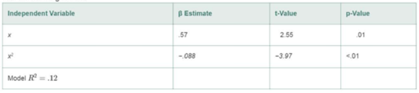
- a. Conduct a test of overall model utility. Use α =.05.
- b. The researchers hypothesized that leadership ability increases at a decreasing rate with assertiveness. Set up the null and alternative hypotheses to test this theory.
- c. Use the reported results to conduct the test, part b. Give your conclusion (at α = .05) in the words of the problem.
Expert Solution & Answer
Want to see the full answer?
Check out a sample textbook solution
Students have asked these similar questions
4.96 The breaking strengths for 1-foot-square samples of a particular synthetic fabric are approximately normally distributed with a mean of 2,250 pounds per square inch (psi) and a standard deviation of 10.2 psi. Find the probability of selecting a 1-foot-square sample of material at random that on testing would have a breaking strength in excess of 2,265 psi.4.97 Refer to Exercise 4.96. Suppose that a new synthetic fabric has been developed that may have a different mean breaking strength. A random sample of 15 1-foot sections is obtained, and each section is tested for breaking strength. If we assume that the population standard deviation for the new fabric is identical to that for the old fabric, describe the sampling distribution forybased on random samples of 15 1-foot sections of new fabric
Une Entreprise œuvrant dans le domaine du multividéo donne l'opportunité à ses
programmeurs-analystes d'évaluer la performance des cadres supérieurs.
Voici les résultats obtenues (sur une échelle de 10 à 50) où 50 représentent une
excellente performance. 10 programmeurs furent sélectionnés au hazard pour
évaluer deux cadres. Un rapport Excel est également fourni.
Programmeurs
Cadre A Cadre B
1
34
36
2
32
34
3
18
19
33
38
19
21
21
23
7
35
34
8
20
20
9
34
34
10
36
34
Test d'égalité des espérances: observations pairées
A television news channel samples 25 gas stations from its local area and uses the results to estimate the average gas price for the state. What’s wrong with its margin of error?
Chapter 12 Solutions
Statistics for Business and Economics (13th Edition)
Ch. 12.3 - Write a first-order model relating E(y) to a. two...Ch. 12.3 - Minitab was used to fit the model E(y) = (0 + 1x1...Ch. 12.3 - Suppose you fit the multiple regression model y =0...Ch. 12.3 - Suppose you fit the first-order multiple...Ch. 12.3 - Prob. 12.5LMCh. 12.3 - Prob. 12.6LMCh. 12.3 - Prob. 12.7LMCh. 12.3 - If the analysis of variance F-test leads to the...Ch. 12.3 - Ambiance of 5-star hotels. Although invisible and...Ch. 12.3 - Forecasting movie revenues with Twitter. Refer to...
Ch. 12.3 - Accounting and Machiavellianism. Refer to the...Ch. 12.3 - Prob. 12.12ACBCh. 12.3 - Predicting elements in aluminum alloys. Aluminum...Ch. 12.3 - Novelty of a vacation destination. Many tourists...Ch. 12.3 - Arsenic in groundwater. Environmental Science ...Ch. 12.3 - Reality TV and cosmetic surgery. How much...Ch. 12.3 - Contamination from a plant's discharge. Refer to...Ch. 12.3 - Cooling method for gas turbines. Refer to the...Ch. 12.3 - Rankings of research universities. Refer to the...Ch. 12.3 - Bubble behavior in subcooled flow boiling. In...Ch. 12.3 - Prob. 12.22ACICh. 12.3 - Prob. 12.23ACACh. 12.3 - Prob. 12.24ACACh. 12.4 - Characteristics of lead users. Refer to the...Ch. 12.4 - Prob. 12.26ACBCh. 12.4 - Reality TV and cosmetic surgery. Refer to the Body...Ch. 12.4 - Chemical plant contamination. Refer to Exercise...Ch. 12.4 - Prob. 12.29ACBCh. 12.4 - Arsenic in groundwater. Refer to the Environmental...Ch. 12.4 - Prob. 12.32ACICh. 12.4 - Prob. 12.33ACICh. 12.4 - Boiler drum production. In a production facility,...Ch. 12.5 - Suppose the true relationship between E(y) and the...Ch. 12.5 - Suppose you fit the interaction model y = 0 + x1 +...Ch. 12.5 - Prob. 12.37LMCh. 12.5 - Tipping behavior in restaurants. Can food servers...Ch. 12.5 - Forecasting movie revenues with Twitter. Refer to...Ch. 12.5 - Prob. 12.41ACBCh. 12.5 - Prob. 12.42ACBCh. 12.5 - Reality TV and cosmetic surgery. Refer to the Body...Ch. 12.5 - Factors that impact an auditors judgment. A study...Ch. 12.5 - Service workers and customer relations. A study in...Ch. 12.5 - Bubble behavior in subcooled flow boiling. Refer...Ch. 12.5 - Arsenic in groundwater. Refer to the Environmental...Ch. 12.5 - Cooling method for gas turbines. Refer to the...Ch. 12.6 - Write a second-order model relating the mean of y,...Ch. 12.6 - Prob. 12.50LMCh. 12.6 - Prob. 12.51LMCh. 12.6 - Prob. 12.52LMCh. 12.6 - Minitab was used to fit the complete second-order...Ch. 12.6 - Personality traits and job performance. When...Ch. 12.6 - Going for it on fourth-down in the NFL. Refer to...Ch. 12.6 - Prob. 12.56ACBCh. 12.6 - Prob. 12.57ACBCh. 12.6 - Assertiveness and leadership. Management...Ch. 12.6 - Goal congruence in top management teams. Do chief...Ch. 12.6 - Prob. 12.60ACICh. 12.6 - Revenues of popular movies. The Internet Movie...Ch. 12.6 - Prob. 12.62ACICh. 12.6 - Prob. 12.63ACICh. 12.6 - Prob. 12.64ACICh. 12.6 - Prob. 12.65ACICh. 12.7 - Write a regression model relating the mean value...Ch. 12.7 - Prob. 12.67LMCh. 12.7 - Prob. 12.68LMCh. 12.7 - Prob. 12.69LMCh. 12.7 - Prob. 12.70ACBCh. 12.7 - Prob. 12.71ACBCh. 12.7 - Prob. 12.72ACBCh. 12.7 - Prob. 12.73ACBCh. 12.7 - Buy-side vs. sell-side analysts earnings...Ch. 12.7 - Prob. 12.75ACBCh. 12.7 - Charisma of top-level leaders. Refer to the...Ch. 12.7 - Corporate sustainability and firm characteristics....Ch. 12.7 - Homework assistance for accounting students. Refer...Ch. 12.7 - Improving driving performance while fatigued....Ch. 12.7 - Prob. 12.80ACACh. 12.7 - Banning controversial sports team sponsors. Refer...Ch. 12.8 - Consider a multiple regression model for a...Ch. 12.8 - Prob. 12.83LMCh. 12.8 - Consider the model: y = 0+ 1x1+ 2 x2+ 3 x3+...Ch. 12.8 - Consider the model:...Ch. 12.8 - Prob. 12.86LMCh. 12.8 - Reality TV and cosmetic surgery. Refer to the Body...Ch. 12.8 - Do blondes raise more funds? Refer to the Economic...Ch. 12.8 - Prob. 12.89ACBCh. 12.8 - Buy-side vs. sell-side analysts earnings...Ch. 12.8 - Workplace bullying and intention to leave....Ch. 12.8 - Agreeableness, gender, and wages. Do agreeable...Ch. 12.8 - Chemical plant contamination. Refer to Exercise...Ch. 12.8 - Prob. 12.94ACICh. 12.8 - Recently sold, single-family homes. The National...Ch. 12.8 - Charisma of top-level leaders Refer to the Academy...Ch. 12.9 - Determine which pairs of the following models are...Ch. 12.9 - Prob. 12.98LMCh. 12.9 - Prob. 12.99LMCh. 12.9 - Shared leadership in airplane crews. Refer to the...Ch. 12.9 - Buy-side vs. sell-side analysts earnings...Ch. 12.9 - Workplace bullying and intention to leave. Refer...Ch. 12.9 - Cooling method for gas turbines. Refer to the...Ch. 12.9 - Prob. 12.104ACBCh. 12.9 - Reality TV and cosmetic surgery. Refer to the Body...Ch. 12.9 - Study of supervisor-targeted aggression....Ch. 12.9 - Prob. 12.107ACICh. 12.9 - Recently sold, single-family homes. Refer to the...Ch. 12.9 - Prob. 12.109ACICh. 12.9 - Prob. 12.110ACACh. 12.10 - Prob. 12.111LMCh. 12.10 - Teacher pay and pupil performance. In Economic...Ch. 12.10 - Risk management performance. An article in the...Ch. 12.10 - Accuracy of software effort estimates....Ch. 12.10 - Diet of ducks bred for broiling. Corn is high in...Ch. 12.10 - Reality TV and cosmetic surgery. Refer to the Body...Ch. 12.10 - Prob. 12.117ACICh. 12.10 - Prob. 12.118ACICh. 12.10 - Prob. 12.119ACICh. 12.12 - Identify the problem(s) in each of the residual...Ch. 12.12 - Consider fitting the multiple regression model...Ch. 12.12 - Emotional intelligence and team performance. Refer...Ch. 12.12 - State casket sales restrictions. Some states...Ch. 12.12 - Personality traits and job performance. Refer to...Ch. 12.12 - Women in top management. Refer to the Journal of...Ch. 12.12 - Accuracy of software effort estimates. Refer to...Ch. 12.12 - Arsenic in groundwater. Refer to the Environmental...Ch. 12.12 - Reality TV and cosmetic surgery. Refer to the Body...Ch. 12.12 - Failure times of silicon wafer microchips. Refer...Ch. 12.12 - Bubble behavior in subcooled flow boiling. Refer...Ch. 12.12 - Banning controversial sports team sponsors. Refer...Ch. 12.12 - Cooling method for gas turbines. Refer to the...Ch. 12.12 - Agreeableness, gender, and wages. Refer to the...Ch. 12 - Suppose you have developed a regression model to...Ch. 12 - When a multiple regression model is used for...Ch. 12 - Suppose you fit the model y=0+1x1+2x12+3x2+4x1x2+...Ch. 12 - Prob. 12.137LMCh. 12 - Prob. 12.138LMCh. 12 - Prob. 12.139LMCh. 12 - Prob. 12.140LMCh. 12 - Prob. 12.141LMCh. 12 - Prob. 12.142LMCh. 12 - Prob. 12.143LMCh. 12 - Prob. 12.144LMCh. 12 - Comparing private and public college tuition....Ch. 12 - Prob. 12.146ACBCh. 12 - Prob. 12.147ACBCh. 12 - Highway crash data analysis. Researchers at...Ch. 12 - Prob. 12.149ACBCh. 12 - Mental health of a community. An article in the...Ch. 12 - Prob. 12.151ACBCh. 12 - Testing tires for wear. Underinflated or...Ch. 12 - Prob. 12.153ACBCh. 12 - Prob. 12.154ACBCh. 12 - Prob. 12.155ACBCh. 12 - Prob. 12.156ACBCh. 12 - Prob. 12.157ACBCh. 12 - Promotion of supermarket vegetables. A supermarket...Ch. 12 - Yield strength of steel alloy. Industrial...Ch. 12 - Prob. 12.160ACICh. 12 - Prob. 12.161ACICh. 12 - Improving Math SAT scores. Refer to the Chance...Ch. 12 - Prob. 12.163ACICh. 12 - Prob. 12.164ACICh. 12 - Prob. 12.165ACICh. 12 - Prob. 12.166ACICh. 12 - Sale prices of apartments. A Minneapolis,...Ch. 12 - Volatility of foreign stocks. The relationship...Ch. 12 - Prob. 12.169ACICh. 12 - Prob. 12.170ACICh. 12 - State casket sales restrictions Refer to the...Ch. 12 - Modeling monthly collision claims. A medium-sized...Ch. 12 - Developing a model for college GPA. Many colleges...
Knowledge Booster


Learn more about
Need a deep-dive on the concept behind this application? Look no further. Learn more about this topic, statistics and related others by exploring similar questions and additional content below.Similar questions
- You’re fed up with keeping Fido locked inside, so you conduct a mail survey to find out people’s opinions on the new dog barking ordinance in a certain city. Of the 10,000 people who receive surveys, 1,000 respond, and only 80 are in favor of it. You calculate the margin of error to be 1.2 percent. Explain why this reported margin of error is misleading.arrow_forwardYou find out that the dietary scale you use each day is off by a factor of 2 ounces (over — at least that’s what you say!). The margin of error for your scale was plus or minus 0.5 ounces before you found this out. What’s the margin of error now?arrow_forwardSuppose that Sue and Bill each make a confidence interval out of the same data set, but Sue wants a confidence level of 80 percent compared to Bill’s 90 percent. How do their margins of error compare?arrow_forward
- Suppose that you conduct a study twice, and the second time you use four times as many people as you did the first time. How does the change affect your margin of error? (Assume the other components remain constant.)arrow_forwardOut of a sample of 200 babysitters, 70 percent are girls, and 30 percent are guys. What’s the margin of error for the percentage of female babysitters? Assume 95 percent confidence.What’s the margin of error for the percentage of male babysitters? Assume 95 percent confidence.arrow_forwardYou sample 100 fish in Pond A at the fish hatchery and find that they average 5.5 inches with a standard deviation of 1 inch. Your sample of 100 fish from Pond B has the same mean, but the standard deviation is 2 inches. How do the margins of error compare? (Assume the confidence levels are the same.)arrow_forward
- A survey of 1,000 dental patients produces 450 people who floss their teeth adequately. What’s the margin of error for this result? Assume 90 percent confidence.arrow_forwardThe annual aggregate claim amount of an insurer follows a compound Poisson distribution with parameter 1,000. Individual claim amounts follow a Gamma distribution with shape parameter a = 750 and rate parameter λ = 0.25. 1. Generate 20,000 simulated aggregate claim values for the insurer, using a random number generator seed of 955.Display the first five simulated claim values in your answer script using the R function head(). 2. Plot the empirical density function of the simulated aggregate claim values from Question 1, setting the x-axis range from 2,600,000 to 3,300,000 and the y-axis range from 0 to 0.0000045. 3. Suggest a suitable distribution, including its parameters, that approximates the simulated aggregate claim values from Question 1. 4. Generate 20,000 values from your suggested distribution in Question 3 using a random number generator seed of 955. Use the R function head() to display the first five generated values in your answer script. 5. Plot the empirical density…arrow_forwardFind binomial probability if: x = 8, n = 10, p = 0.7 x= 3, n=5, p = 0.3 x = 4, n=7, p = 0.6 Quality Control: A factory produces light bulbs with a 2% defect rate. If a random sample of 20 bulbs is tested, what is the probability that exactly 2 bulbs are defective? (hint: p=2% or 0.02; x =2, n=20; use the same logic for the following problems) Marketing Campaign: A marketing company sends out 1,000 promotional emails. The probability of any email being opened is 0.15. What is the probability that exactly 150 emails will be opened? (hint: total emails or n=1000, x =150) Customer Satisfaction: A survey shows that 70% of customers are satisfied with a new product. Out of 10 randomly selected customers, what is the probability that at least 8 are satisfied? (hint: One of the keyword in this question is “at least 8”, it is not “exactly 8”, the correct formula for this should be = 1- (binom.dist(7, 10, 0.7, TRUE)). The part in the princess will give you the probability of seven and less than…arrow_forward
- please answer these questionsarrow_forwardSelon une économiste d’une société financière, les dépenses moyennes pour « meubles et appareils de maison » ont été moins importantes pour les ménages de la région de Montréal, que celles de la région de Québec. Un échantillon aléatoire de 14 ménages pour la région de Montréal et de 16 ménages pour la région Québec est tiré et donne les données suivantes, en ce qui a trait aux dépenses pour ce secteur d’activité économique. On suppose que les données de chaque population sont distribuées selon une loi normale. Nous sommes intéressé à connaitre si les variances des populations sont égales.a) Faites le test d’hypothèse sur deux variances approprié au seuil de signification de 1 %. Inclure les informations suivantes : i. Hypothèse / Identification des populationsii. Valeur(s) critique(s) de Fiii. Règle de décisioniv. Valeur du rapport Fv. Décision et conclusion b) A partir des résultats obtenus en a), est-ce que l’hypothèse d’égalité des variances pour cette…arrow_forwardAccording to an economist from a financial company, the average expenditures on "furniture and household appliances" have been lower for households in the Montreal area than those in the Quebec region. A random sample of 14 households from the Montreal region and 16 households from the Quebec region was taken, providing the following data regarding expenditures in this economic sector. It is assumed that the data from each population are distributed normally. We are interested in knowing if the variances of the populations are equal. a) Perform the appropriate hypothesis test on two variances at a significance level of 1%. Include the following information: i. Hypothesis / Identification of populations ii. Critical F-value(s) iii. Decision rule iv. F-ratio value v. Decision and conclusion b) Based on the results obtained in a), is the hypothesis of equal variances for this socio-economic characteristic measured in these two populations upheld? c) Based on the results obtained in a),…arrow_forward
arrow_back_ios
SEE MORE QUESTIONS
arrow_forward_ios
Recommended textbooks for you
 Big Ideas Math A Bridge To Success Algebra 1: Stu...AlgebraISBN:9781680331141Author:HOUGHTON MIFFLIN HARCOURTPublisher:Houghton Mifflin Harcourt
 Functions and Change: A Modeling Approach to Coll...AlgebraISBN:9781337111348Author:Bruce Crauder, Benny Evans, Alan NoellPublisher:Cengage Learning
 Glencoe Algebra 1, Student Edition, 9780079039897...AlgebraISBN:9780079039897Author:CarterPublisher:McGraw Hill
Big Ideas Math A Bridge To Success Algebra 1: Stu...
Algebra
ISBN:9781680331141
Author:HOUGHTON MIFFLIN HARCOURT
Publisher:Houghton Mifflin Harcourt
Functions and Change: A Modeling Approach to Coll...
Algebra
ISBN:9781337111348
Author:Bruce Crauder, Benny Evans, Alan Noell
Publisher:Cengage Learning
Glencoe Algebra 1, Student Edition, 9780079039897...
Algebra
ISBN:9780079039897
Author:Carter
Publisher:McGraw Hill
Time Series Analysis Theory & Uni-variate Forecasting Techniques; Author: Analytics University;https://www.youtube.com/watch?v=_X5q9FYLGxM;License: Standard YouTube License, CC-BY
Operations management 101: Time-series, forecasting introduction; Author: Brandoz Foltz;https://www.youtube.com/watch?v=EaqZP36ool8;License: Standard YouTube License, CC-BY