
Videos
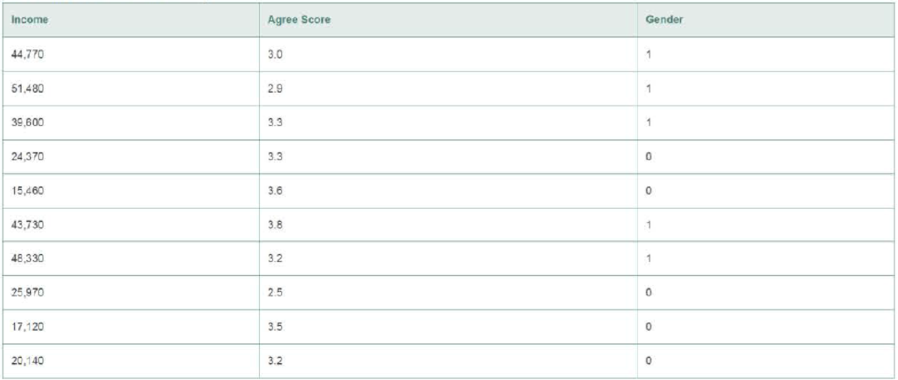
Agreeableness, gender, and wages. Do agreeable individuals get paid less, on average, than those who are less agreeable on the job? And is this gap greater for males than for females? These questions were addressed in the Journal of Personality and Social Psychology (February 2012). Several variables were measured for each in a sample of individuals enrolled in the National Survey of Midlife Development in the U.S. Three of these variables are: (1) level of agreeableness score (where higher scores indicate a greater level of agreeableness). (2) gender (male or female). and (3) annual income (dollars). The researchers modeled mean income. E(y) , as a
Data for First 10 Individuals in Study
- a. Consider the model, E(y)=β0+β1x1+ β2x2 The researchers theorized that for either gender, income would decrease as agreeableness score increases. If this theory is true, what is the expected sign of β1 in the model?
- b. The researchers also theorized that the rate of decrease of income with agreeableness score would be steeper for males than for females (i.e., the income gap between males and females would be greater the less agreeable the individuals are). Can this theory be tested using the model, part a? Explain.
- c. Consider the interaction model, E(y)=β0+β1x1+ β2x2+β3x1x2. If the theory, part b, is true, give the expected sign of β1. The expected sign of β3.
- d. Fit the model, part c, to the sample data. Check the signs of the estimated β coefficients. How do they compare with the
expected values , part c? - e. Refer to the interaction model, part c. Give the null and alternative hypotheses for testing whether the rate of decrease of income with agreeableness score is steeper for males than for females.
- f. Conduct the test, part e. Use α = .05. Is the researchers’ theory supported?
Want to see the full answer?
Check out a sample textbook solution
Chapter 12 Solutions
Statistics for Business and Economics (13th Edition)


- Question 1 The data shown in Table 1 are and R values for 24 samples of size n = 5 taken from a process producing bearings. The measurements are made on the inside diameter of the bearing, with only the last three decimals recorded (i.e., 34.5 should be 0.50345). Table 1: Bearing Diameter Data Sample Number I R Sample Number I R 1 34.5 3 13 35.4 8 2 34.2 4 14 34.0 6 3 31.6 4 15 37.1 5 4 31.5 4 16 34.9 7 5 35.0 5 17 33.5 4 6 34.1 6 18 31.7 3 7 32.6 4 19 34.0 8 8 33.8 3 20 35.1 9 34.8 7 21 33.7 2 10 33.6 8 22 32.8 1 11 31.9 3 23 33.5 3 12 38.6 9 24 34.2 2 (a) Set up and R charts on this process. Does the process seem to be in statistical control? If necessary, revise the trial control limits. [15 pts] (b) If specifications on this diameter are 0.5030±0.0010, find the percentage of nonconforming bearings pro- duced by this process. Assume that diameter is normally distributed. [10 pts] 1arrow_forward4. (5 pts) Conduct a chi-square contingency test (test of independence) to assess whether there is an association between the behavior of the elderly person (did not stop to talk, did stop to talk) and their likelihood of falling. Below, please state your null and alternative hypotheses, calculate your expected values and write them in the table, compute the test statistic, test the null by comparing your test statistic to the critical value in Table A (p. 713-714) of your textbook and/or estimating the P-value, and provide your conclusions in written form. Make sure to show your work. Did not stop walking to talk Stopped walking to talk Suffered a fall 12 11 Totals 23 Did not suffer a fall | 2 Totals 35 37 14 46 60 Tarrow_forwardQuestion 2 Parts manufactured by an injection molding process are subjected to a compressive strength test. Twenty samples of five parts each are collected, and the compressive strengths (in psi) are shown in Table 2. Table 2: Strength Data for Question 2 Sample Number x1 x2 23 x4 x5 R 1 83.0 2 88.6 78.3 78.8 3 85.7 75.8 84.3 81.2 78.7 75.7 77.0 71.0 84.2 81.0 79.1 7.3 80.2 17.6 75.2 80.4 10.4 4 80.8 74.4 82.5 74.1 75.7 77.5 8.4 5 83.4 78.4 82.6 78.2 78.9 80.3 5.2 File Preview 6 75.3 79.9 87.3 89.7 81.8 82.8 14.5 7 74.5 78.0 80.8 73.4 79.7 77.3 7.4 8 79.2 84.4 81.5 86.0 74.5 81.1 11.4 9 80.5 86.2 76.2 64.1 80.2 81.4 9.9 10 75.7 75.2 71.1 82.1 74.3 75.7 10.9 11 80.0 81.5 78.4 73.8 78.1 78.4 7.7 12 80.6 81.8 79.3 73.8 81.7 79.4 8.0 13 82.7 81.3 79.1 82.0 79.5 80.9 3.6 14 79.2 74.9 78.6 77.7 75.3 77.1 4.3 15 85.5 82.1 82.8 73.4 71.7 79.1 13.8 16 78.8 79.6 80.2 79.1 80.8 79.7 2.0 17 82.1 78.2 18 84.5 76.9 75.5 83.5 81.2 19 79.0 77.8 20 84.5 73.1 78.2 82.1 79.2 81.1 7.6 81.2 84.4 81.6 80.8…arrow_forward
- Name: Lab Time: Quiz 7 & 8 (Take Home) - due Wednesday, Feb. 26 Contingency Analysis (Ch. 9) In lab 5, part 3, you will create a mosaic plot and conducted a chi-square contingency test to evaluate whether elderly patients who did not stop walking to talk (vs. those who did stop) were more likely to suffer a fall in the next six months. I have tabulated the data below. Answer the questions below. Please show your calculations on this or a separate sheet. Did not stop walking to talk Stopped walking to talk Totals Suffered a fall Did not suffer a fall Totals 12 11 23 2 35 37 14 14 46 60 Quiz 7: 1. (2 pts) Compute the odds of falling for each group. Compute the odds ratio for those who did not stop walking vs. those who did stop walking. Interpret your result verbally.arrow_forwardSolve please and thank you!arrow_forward7. In a 2011 article, M. Radelet and G. Pierce reported a logistic prediction equation for the death penalty verdicts in North Carolina. Let Y denote whether a subject convicted of murder received the death penalty (1=yes), for the defendant's race h (h1, black; h = 2, white), victim's race i (i = 1, black; i = 2, white), and number of additional factors j (j = 0, 1, 2). For the model logit[P(Y = 1)] = a + ß₁₂ + By + B²², they reported = -5.26, D â BD = 0, BD = 0.17, BY = 0, BY = 0.91, B = 0, B = 2.02, B = 3.98. (a) Estimate the probability of receiving the death penalty for the group most likely to receive it. [4 pts] (b) If, instead, parameters used constraints 3D = BY = 35 = 0, report the esti- mates. [3 pts] h (c) If, instead, parameters used constraints Σ₁ = Σ₁ BY = Σ; B = 0, report the estimates. [3 pts] Hint the probabilities, odds and odds ratios do not change with constraints.arrow_forward
- Solve please and thank you!arrow_forwardSolve please and thank you!arrow_forwardQuestion 1:We want to evaluate the impact on the monetary economy for a company of two types of strategy (competitive strategy, cooperative strategy) adopted by buyers.Competitive strategy: strategy characterized by firm behavior aimed at obtaining concessions from the buyer.Cooperative strategy: a strategy based on a problem-solving negotiating attitude, with a high level of trust and cooperation.A random sample of 17 buyers took part in a negotiation experiment in which 9 buyers adopted the competitive strategy, and the other 8 the cooperative strategy. The savings obtained for each group of buyers are presented in the pdf that i sent: For this problem, we assume that the samples are random and come from two normal populations of unknown but equal variances.According to the theory, the average saving of buyers adopting a competitive strategy will be lower than that of buyers adopting a cooperative strategy.a) Specify the population identifications and the hypotheses H0 and H1…arrow_forward
- You assume that the annual incomes for certain workers are normal with a mean of $28,500 and a standard deviation of $2,400. What’s the chance that a randomly selected employee makes more than $30,000?What’s the chance that 36 randomly selected employees make more than $30,000, on average?arrow_forwardWhat’s the chance that a fair coin comes up heads more than 60 times when you toss it 100 times?arrow_forwardSuppose that you have a normal population of quiz scores with mean 40 and standard deviation 10. Select a random sample of 40. What’s the chance that the mean of the quiz scores won’t exceed 45?Select one individual from the population. What’s the chance that his/her quiz score won’t exceed 45?arrow_forward
 Glencoe Algebra 1, Student Edition, 9780079039897...AlgebraISBN:9780079039897Author:CarterPublisher:McGraw Hill
 Big Ideas Math A Bridge To Success Algebra 1: Stu...AlgebraISBN:9781680331141Author:HOUGHTON MIFFLIN HARCOURTPublisher:Houghton Mifflin Harcourt
 Holt Mcdougal Larson Pre-algebra: Student Edition...AlgebraISBN:9780547587776Author:HOLT MCDOUGALPublisher:HOLT MCDOUGAL
 Functions and Change: A Modeling Approach to Coll...AlgebraISBN:9781337111348Author:Bruce Crauder, Benny Evans, Alan NoellPublisher:Cengage Learning
 College Algebra (MindTap Course List)AlgebraISBN:9781305652231Author:R. David Gustafson, Jeff HughesPublisher:Cengage Learning