Chapter 12.3, Problem 12.13ACB

Predicting elements in aluminum alloys. Aluminum scraps that are recycled into alloys are classified into three categories: soft-drink cans, pots and pans, and automobile crank chambers. A study of how these three materials affect the metal elements present in aluminum alloys was published in Advances in Applied Physics (Vol. 1, 2013). Data on 126 production runs at an aluminum plant were used to model the percentage (y) of various elements (e.g., silver, boron, iron) that make up the aluminum alloy. Three independent variables were used in the model: x₁ = proportion of aluminum scraps from cans, x₂ = proportion of aluminum scraps from pots/pans, and x₃ = proportion of aluminum scraps from crank chambers. The first-order model, E (y) = β_{0 +} β₁ x_{1 +} β₂x_{2 +} β₃x₃, was fit to the data for several elements. The estimates of the model parameters (p-values in parentheses) for silver and iron are shown in the accompanying table.

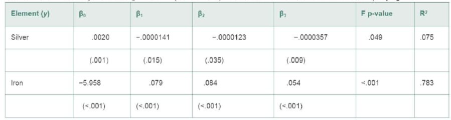
1. a. Is the overall model statistically useful (at α = .05) for predicting the percentage of silver in the alloy? If so, give a practical interpretation of R².
2. b. Is the overall model statistically useful (at α = .05) for predicting the percentage of iron in the alloy? If so, give a practical interpretation of R².
3. c. Based on the parameter estimates, sketch the relationship between percentage of silver (y) and proportion of aluminum scraps from cans (x₁). Conduct a test to determine if this relationship is statistically significant at α = .05
4. d. Based on the parameter estimates, sketch the relationship between percentage of iron (y) and proportion of aluminum scraps from cans (x₁). Conduct a test to determine if this relationship is statistically significant at α = .05