
Videos
An accurate assessment of oxygen consumption provides important information for determining energy expenditure requirements for physically demanding tasks. The paper “Oxygen Consumption During Fire Suppression: Error of Heart Rate Estimation” (Ergonomics [1991]: 1469–1474) reported on a study in which x = Oxygen consumption (in milliliters per kilogram per minute) during a treadmill test was determined for a sample of 10 firefighters. Then y = Oxygen consumption at a comparable heart rate was measured for each of the 10 individuals while they performed a fire-suppression simulation. This resulted in the following data and

- a. Does the scatterplot suggest an approximate linear relationship?
- b. The investigators fit a least-squares line. The resulting Minitab output is given in the following:
The regression equation is firecon = 211. 4 + 1. 09 treadcon
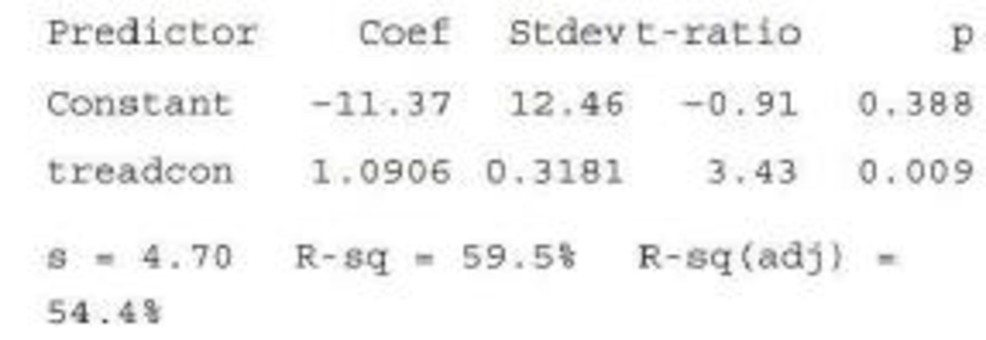
Predict fire-simulation consumption when treadmill consumption is 40.
- c. How effectively does a straight line summarize the relationship?
- d. Delete the first observation, (51.3, 49.3), and calculate the new equation of the least-squares line and the value of r2. What do you conclude? (Hint: For the original data, Σx = 388.8, Σy = 310 .3, Σx2 = 15,338.54, Σxy = 12,306.58, and Σy2 = 10,072.41.)
a.
Discuss whether the scatterplot indicates an approximate linear relationship.
Answer to Problem 66CR
No, the scatterplot does not indicate an approximate linear relationship.
Explanation of Solution
The data relates the oxygen consumption (milliliters per kilogram per minute) of 10 firefighters during a fire-suppression simulation, y to that during a treadmill test, x. The scatterplot between the two variables is given.
Denote the estimated response variable as
A careful inspection of the given scatterplot shows that the points do not fall on a straight line. Rather, the points are scattered almost in a random manner, without showing any pattern in particular. However, there is one extreme point, which is far away from the remaining points. This extreme point appears to provide an impression that there might be a linear relationship between the two variables. Once this point is ignored, it is clear that no such relationship can be determined.
Thus, the scatterplot does not indicate an approximate linear relationship.
b.
Predict the fire-simulation oxygen consumption, if the treadmill oxygen consumption is 40.
Answer to Problem 66CR
The fire-simulation oxygen consumption, when the treadmill oxygen consumption is 40 is 32.254 milliliters per kilogram per minute.
Explanation of Solution
Calculation:
The MINITAB output for the fitting of a least-squares regression line to the given data is given.
In the given output, the column of “Coef” gives the coefficients corresponding to the variables given in the column of “Predictor”. The term “Constant” under the column of ‘Predictor’ gives the intercept of the equation; the term “treadcon” denotes the oxygen consumption of during the treadmill test, x.
Using the values in the output, the equation of the least-squares regression line is
For a treadmill oxygen consumption of 40 milliliters per kilogram per minute,
Thus, the fire-simulation oxygen consumption, when the treadmill oxygen consumption is 40 is 32.254 milliliters per kilogram per minute.
c.
Explain the effectivity of the straight line to summarize the relationship between the variables.
Explanation of Solution
In the given output, the value of
Now,
Thus, it can be interpreted that the oxygen consumption during the treadmill test can predict about 59.5% of the variability in the oxygen consumption during the fire-suppression simulation.
This suggests that the straight line is moderately effective in summarizing the relationship between the variables.
d.
Find the equation of the least-squares line and the value of
Answer to Problem 66CR
The equation of the least-squares line after deleting the first observation, (51.3, 49.3) is
The value of
Explanation of Solution
Calculation:
It is given that, for the original data set,
For the first observation,
Now, the lest-squares regression line is of the form:
Using this formula and the values obtained above, b and a are respectively obtained as follows:
Now,
Thus,
Using the values of a and b obtained above, the equation of the least-squares line after deleting the first observation, (51.3, 49.3) is
Now, it is known that the slope for the least-squares regression of y on x, that is, b can be given by the formula:
Now, it can be shown that:
Similarly,
Thus,
Using the values obtained above, the value of r can be calculated as follows:
It is known that
Hence, the value of
Now,
Now,
Thus, it can be interpreted that the oxygen consumption during the treadmill test can predict about 2% of the variability in the oxygen consumption during the fire-suppression simulation, which is a very low percentage.
Thus, the model 9is not a very good fit for the data.
Want to see more full solutions like this?
Chapter 5 Solutions
Introduction to Statistics and Data Analysis
Additional Math Textbook Solutions
Calculus: Early Transcendentals (2nd Edition)
Precalculus
APPLIED STAT.IN BUS.+ECONOMICS
Elementary Statistics: Picturing the World (7th Edition)
College Algebra (Collegiate Math)


- You find out that the dietary scale you use each day is off by a factor of 2 ounces (over — at least that’s what you say!). The margin of error for your scale was plus or minus 0.5 ounces before you found this out. What’s the margin of error now?arrow_forwardSuppose that Sue and Bill each make a confidence interval out of the same data set, but Sue wants a confidence level of 80 percent compared to Bill’s 90 percent. How do their margins of error compare?arrow_forwardSuppose that you conduct a study twice, and the second time you use four times as many people as you did the first time. How does the change affect your margin of error? (Assume the other components remain constant.)arrow_forward
- Out of a sample of 200 babysitters, 70 percent are girls, and 30 percent are guys. What’s the margin of error for the percentage of female babysitters? Assume 95 percent confidence.What’s the margin of error for the percentage of male babysitters? Assume 95 percent confidence.arrow_forwardYou sample 100 fish in Pond A at the fish hatchery and find that they average 5.5 inches with a standard deviation of 1 inch. Your sample of 100 fish from Pond B has the same mean, but the standard deviation is 2 inches. How do the margins of error compare? (Assume the confidence levels are the same.)arrow_forwardA survey of 1,000 dental patients produces 450 people who floss their teeth adequately. What’s the margin of error for this result? Assume 90 percent confidence.arrow_forward
- The annual aggregate claim amount of an insurer follows a compound Poisson distribution with parameter 1,000. Individual claim amounts follow a Gamma distribution with shape parameter a = 750 and rate parameter λ = 0.25. 1. Generate 20,000 simulated aggregate claim values for the insurer, using a random number generator seed of 955.Display the first five simulated claim values in your answer script using the R function head(). 2. Plot the empirical density function of the simulated aggregate claim values from Question 1, setting the x-axis range from 2,600,000 to 3,300,000 and the y-axis range from 0 to 0.0000045. 3. Suggest a suitable distribution, including its parameters, that approximates the simulated aggregate claim values from Question 1. 4. Generate 20,000 values from your suggested distribution in Question 3 using a random number generator seed of 955. Use the R function head() to display the first five generated values in your answer script. 5. Plot the empirical density…arrow_forwardFind binomial probability if: x = 8, n = 10, p = 0.7 x= 3, n=5, p = 0.3 x = 4, n=7, p = 0.6 Quality Control: A factory produces light bulbs with a 2% defect rate. If a random sample of 20 bulbs is tested, what is the probability that exactly 2 bulbs are defective? (hint: p=2% or 0.02; x =2, n=20; use the same logic for the following problems) Marketing Campaign: A marketing company sends out 1,000 promotional emails. The probability of any email being opened is 0.15. What is the probability that exactly 150 emails will be opened? (hint: total emails or n=1000, x =150) Customer Satisfaction: A survey shows that 70% of customers are satisfied with a new product. Out of 10 randomly selected customers, what is the probability that at least 8 are satisfied? (hint: One of the keyword in this question is “at least 8”, it is not “exactly 8”, the correct formula for this should be = 1- (binom.dist(7, 10, 0.7, TRUE)). The part in the princess will give you the probability of seven and less than…arrow_forwardplease answer these questionsarrow_forward
- Selon une économiste d’une société financière, les dépenses moyennes pour « meubles et appareils de maison » ont été moins importantes pour les ménages de la région de Montréal, que celles de la région de Québec. Un échantillon aléatoire de 14 ménages pour la région de Montréal et de 16 ménages pour la région Québec est tiré et donne les données suivantes, en ce qui a trait aux dépenses pour ce secteur d’activité économique. On suppose que les données de chaque population sont distribuées selon une loi normale. Nous sommes intéressé à connaitre si les variances des populations sont égales.a) Faites le test d’hypothèse sur deux variances approprié au seuil de signification de 1 %. Inclure les informations suivantes : i. Hypothèse / Identification des populationsii. Valeur(s) critique(s) de Fiii. Règle de décisioniv. Valeur du rapport Fv. Décision et conclusion b) A partir des résultats obtenus en a), est-ce que l’hypothèse d’égalité des variances pour cette…arrow_forwardAccording to an economist from a financial company, the average expenditures on "furniture and household appliances" have been lower for households in the Montreal area than those in the Quebec region. A random sample of 14 households from the Montreal region and 16 households from the Quebec region was taken, providing the following data regarding expenditures in this economic sector. It is assumed that the data from each population are distributed normally. We are interested in knowing if the variances of the populations are equal. a) Perform the appropriate hypothesis test on two variances at a significance level of 1%. Include the following information: i. Hypothesis / Identification of populations ii. Critical F-value(s) iii. Decision rule iv. F-ratio value v. Decision and conclusion b) Based on the results obtained in a), is the hypothesis of equal variances for this socio-economic characteristic measured in these two populations upheld? c) Based on the results obtained in a),…arrow_forwardA major company in the Montreal area, offering a range of engineering services from project preparation to construction execution, and industrial project management, wants to ensure that the individuals who are responsible for project cost estimation and bid preparation demonstrate a certain uniformity in their estimates. The head of civil engineering and municipal services decided to structure an experimental plan to detect if there could be significant differences in project evaluation. Seven projects were selected, each of which had to be evaluated by each of the two estimators, with the order of the projects submitted being random. The obtained estimates are presented in the table below. a) Complete the table above by calculating: i. The differences (A-B) ii. The sum of the differences iii. The mean of the differences iv. The standard deviation of the differences b) What is the value of the t-statistic? c) What is the critical t-value for this test at a significance level of 1%?…arrow_forward
 Glencoe Algebra 1, Student Edition, 9780079039897...AlgebraISBN:9780079039897Author:CarterPublisher:McGraw Hill