
Introduction to Statistics and Data Analysis
5th Edition
ISBN: 9781305115347
Author: Roxy Peck; Chris Olsen; Jay L. Devore
Publisher: Brooks Cole
expand_more
expand_more
format_list_bulleted
Concept explainers
Videos
Textbook Question
Chapter 5.3, Problem 40E
The article referenced in the previous exercise also gave data on the percentage of operating costs covered by park revenues for the 2007–2008 fiscal year.
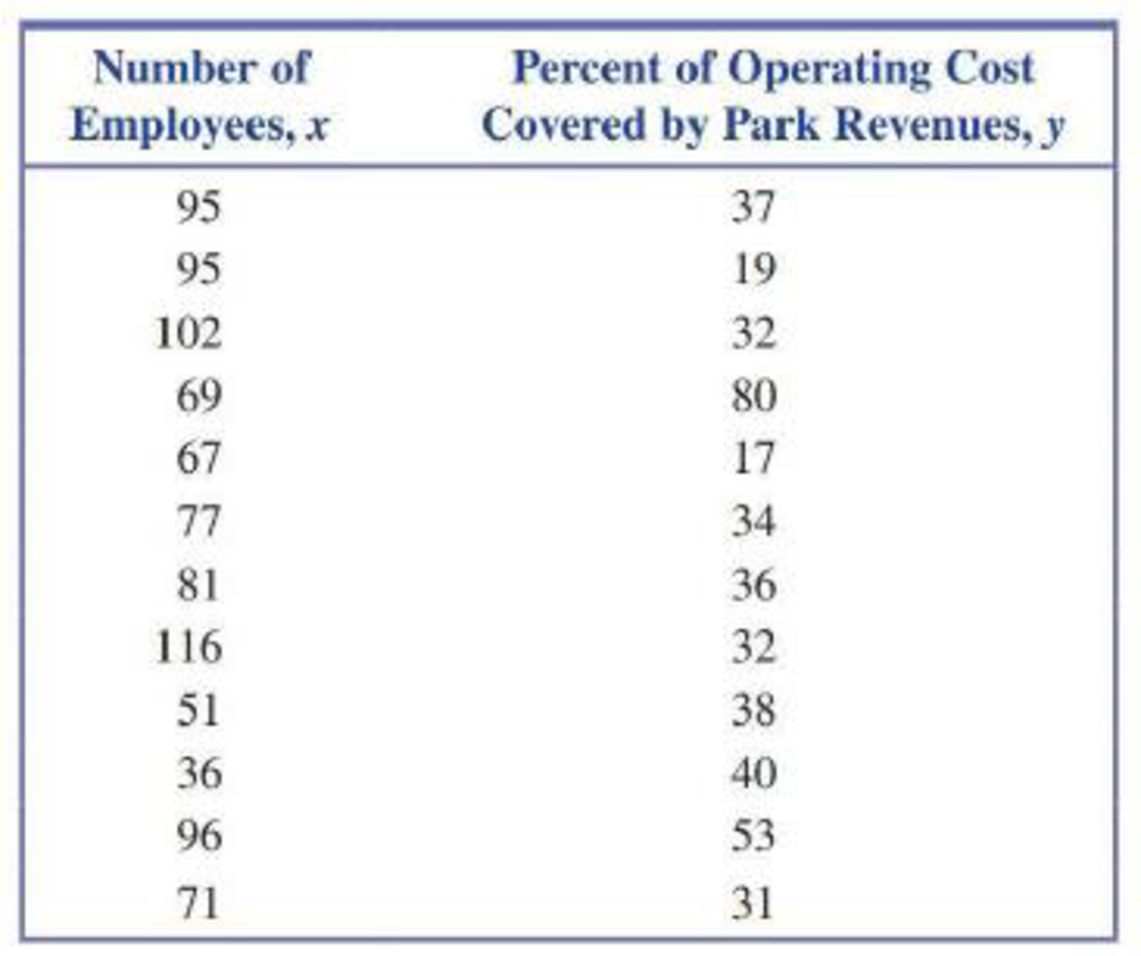
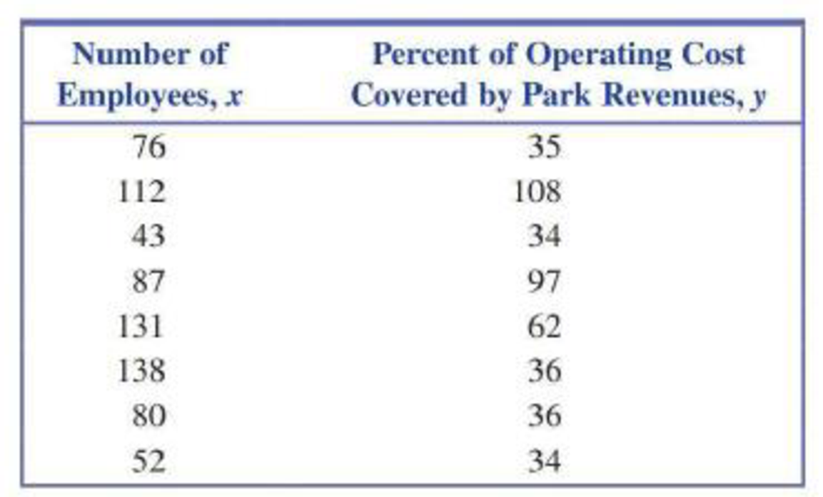
- a. Find the equation of the least-squares line relating y = Percent of operating costs covered by park revenues and x = Number of employees.
- b. Based on the values of r2 and se, do you think that the least-squares line does a good job of describing the relationship between y = Percent of operating costs covered by park revenues and x = Number of employees? Explain.
- c. The graph at the bottom of the page is a
scatterplot of y = Percent of operating costs covered by park revenues and x = Number of employees. The least-squares line is also shown. Which observations are outliers? Do the observations with the largest residuals correspond to the park districts with the largest number of employees?
Expert Solution & Answer
Want to see the full answer?
Check out a sample textbook solution
Students have asked these similar questions
3. Please
What does the margin of error include? When a margin of error is reported for a survey, it includes
a. random sampling error and other practical difficulties like undercoverage and non-response
b. random sampling error, but not other practical difficulties like undercoverage and nonresponse
c. practical difficulties like undercoverage and nonresponse, but not random smapling error
d. none of the above is corret
solve part a on paper
Chapter 5 Solutions
Introduction to Statistics and Data Analysis
Ch. 5.1 - For each of the scatterplots shown, answer the...Ch. 5.1 - For each of the following pairs of variables,...Ch. 5.1 - Is the following statement correct? Explain why or...Ch. 5.1 - Prob. 4ECh. 5.1 - Prob. 5ECh. 5.1 - The accompanying data are x = Cost (cents per...Ch. 5.1 - The authors of the paper Flat-footedness Is Not a...Ch. 5.1 - Prob. 8ECh. 5.1 - Prob. 9ECh. 5.1 - The accompanying data were read from graphs that...
Ch. 5.1 - It may seem odd, but one of the ways biologists...Ch. 5.1 - An auction house released a list of 25 recently...Ch. 5.1 - A sample of automobiles traversing a certain...Ch. 5.2 - Two scatterplots are shown below. Explain why it...Ch. 5.2 - The authors of the paper Statistical Methods for...Ch. 5.2 - Prob. 16ECh. 5.2 - A sample of 548 ethnically diverse students from...Ch. 5.2 - The relationship between hospital patient-to-nurse...Ch. 5.2 - Prob. 19ECh. 5.2 - Prob. 20ECh. 5.2 - Studies have shown that people who suffer sudden...Ch. 5.2 - The data given in the previous exercise on x =...Ch. 5.2 - An article on the cost of housing in Califomia...Ch. 5.2 - The following data on sale price, size, and...Ch. 5.2 - Explain why it can be dangerous to use the...Ch. 5.2 - The sales manager of a large company selected a...Ch. 5.2 - Explain why the slope b of the least-squares line...Ch. 5.2 - Prob. 28ECh. 5.3 - Does it pay to stay in school? The report Trends...Ch. 5.3 - The data in the accompanying table is from the...Ch. 5.3 - Prob. 31ECh. 5.3 - Prob. 32ECh. 5.3 - Some types of algae have the potential to cause...Ch. 5.3 - Prob. 34ECh. 5.3 - Prob. 35ECh. 5.3 - Prob. 36ECh. 5.3 - The article Examined Life: What Stanley H. Kaplan...Ch. 5.3 - Prob. 38ECh. 5.3 - The article California State Parks Closure List...Ch. 5.3 - The article referenced in the previous exercise...Ch. 5.3 - A study was carried out to investigate the...Ch. 5.3 - Both r2 and se are used to assess the fit of a...Ch. 5.3 - Prob. 43ECh. 5.4 - Prob. 44ECh. 5.4 - The paper Aspects of Food Finding by Wintering...Ch. 5.4 - Food intake of grazing animals is limited by the...Ch. 5.4 - Prob. 47ECh. 5.4 - Prob. 48ECh. 5.4 - The paper Population Pressure and Agricultural...Ch. 5.4 - Determining the age of an animal can sometimes be...Ch. 5.5 - The paper How Lead Exposure Relates to Temporal...Ch. 5.5 - The following quote is from the paper Evaluation...Ch. 5 - The accompanying data represent x = Amount of...Ch. 5 - The paper A Cross-National Relationship Between...Ch. 5 - The following data on x = Score on a measure of...Ch. 5 - Prob. 58CRCh. 5 - Prob. 59CRCh. 5 - Prob. 60CRCh. 5 - The paper Effects of Canine Parvovirus (CPV) on...Ch. 5 - The paper Aspects of Food Finding by Wintering...Ch. 5 - Data on salmon availability (x) and the percentage...Ch. 5 - No tortilla chip lover likes soggy chips, so it is...Ch. 5 - The article Reduction is Soluble Protein and...Ch. 5 - An accurate assessment of oxygen consumption...Ch. 5 - Consider the four (x, y) pairs (0, 0), (1, 1), 1,...Ch. 5 - Prob. 1CRECh. 5 - Data from a survey of 1046 adults age 50 and older...Ch. 5 - Prob. 3CRECh. 5 - Prob. 4CRECh. 5 - Prob. 5CRECh. 5 - In August 2009, Harris Interactive released the...Ch. 5 - Prob. 7CRECh. 5 - Prob. 8CRECh. 5 - Prob. 9CRECh. 5 - Prob. 10CRECh. 5 - Prob. 11CRECh. 5 - Prob. 12CRECh. 5 - Prob. 13CRECh. 5 - Cost-to-charge ratios (the percentage of the...Ch. 5 - Prob. 15CRECh. 5 - In the article Reproductive Biology of the Aquatic...Ch. 5 - Prob. 17CRECh. 5 - Prob. 18CRECh. 5 - The paper “Population Pressure and Agricultural...Ch. 5 - Anabolic steroid abuse has been increasing despite...Ch. 5 - Prob. 69ECh. 5 - Prob. 70ECh. 5 - Prob. 71ECh. 5 - Prob. 72ECh. 5 - Suppose the hypothetical data below are from a...Ch. 5 - Prob. 74E
Knowledge Booster


Learn more about
Need a deep-dive on the concept behind this application? Look no further. Learn more about this topic, statistics and related others by exploring similar questions and additional content below.Similar questions
- T1.4: Let ẞ(G) be the minimum size of a vertex cover, a(G) be the maximum size of an independent set and m(G) = |E(G)|. (i) Prove that if G is triangle free (no induced K3) then m(G) ≤ a(G)B(G). Hints - The neighborhood of a vertex in a triangle free graph must be independent; all edges have at least one end in a vertex cover. (ii) Show that all graphs of order n ≥ 3 and size m> [n2/4] contain a triangle. Hints - you may need to use either elementary calculus or the arithmetic-geometric mean inequality.arrow_forwardWe consider the one-period model studied in class as an example. Namely, we assumethat the current stock price is S0 = 10. At time T, the stock has either moved up toSt = 12 (with probability p = 0.6) or down towards St = 8 (with probability 1−p = 0.4).We consider a call option on this stock with maturity T and strike price K = 10. Theinterest rate on the money market is zero.As in class, we assume that you, as a customer, are willing to buy the call option on100 shares of stock for $120. The investor, who sold you the option, can adopt one of thefollowing strategies: Strategy 1: (seen in class) Buy 50 shares of stock and borrow $380. Strategy 2: Buy 55 shares of stock and borrow $430. Strategy 3: Buy 60 shares of stock and borrow $480. Strategy 4: Buy 40 shares of stock and borrow $280.(a) For each of strategies 2-4, describe the value of the investor’s portfolio at time 0,and at time T for each possible movement of the stock.(b) For each of strategies 2-4, does the investor have…arrow_forwardNegate the following compound statement using De Morgans's laws.arrow_forward
- Negate the following compound statement using De Morgans's laws.arrow_forwardQuestion 6: Negate the following compound statements, using De Morgan's laws. A) If Alberta was under water entirely then there should be no fossil of mammals.arrow_forwardNegate the following compound statement using De Morgans's laws.arrow_forward
- Characterize (with proof) all connected graphs that contain no even cycles in terms oftheir blocks.arrow_forwardLet G be a connected graph that does not have P4 or C3 as an induced subgraph (i.e.,G is P4, C3 free). Prove that G is a complete bipartite grapharrow_forwardProve sufficiency of the condition for a graph to be bipartite that is, prove that if G hasno odd cycles then G is bipartite as follows:Assume that the statement is false and that G is an edge minimal counterexample. That is, Gsatisfies the conditions and is not bipartite but G − e is bipartite for any edge e. (Note thatthis is essentially induction, just using different terminology.) What does minimality say aboutconnectivity of G? Can G − e be disconnected? Explain why if there is an edge between twovertices in the same part of a bipartition of G − e then there is an odd cyclearrow_forward
arrow_back_ios
SEE MORE QUESTIONS
arrow_forward_ios
Recommended textbooks for you
 Algebra & Trigonometry with Analytic GeometryAlgebraISBN:9781133382119Author:SwokowskiPublisher:Cengage
Algebra & Trigonometry with Analytic Geometry
Algebra
ISBN:9781133382119
Author:Swokowski
Publisher:Cengage
Correlation Vs Regression: Difference Between them with definition & Comparison Chart; Author: Key Differences;https://www.youtube.com/watch?v=Ou2QGSJVd0U;License: Standard YouTube License, CC-BY
Correlation and Regression: Concepts with Illustrative examples; Author: LEARN & APPLY : Lean and Six Sigma;https://www.youtube.com/watch?v=xTpHD5WLuoA;License: Standard YouTube License, CC-BY