
Concept explainers
a)
To determine: The fraction defective in each sample.
Introduction: Quality is a measure of excellence or a state of being free from deficiencies, defects and important variations. It is obtained by consistent and strict commitment to certain standards to attain uniformity of a product to satisfy consumers’ requirement.
a)
Answer to Problem 5P
Explanation of Solution
Given information:
| Sample | 1 | 2 | 3 | 4 |
| Number with errors | 4 | 2 | 5 | 9 |
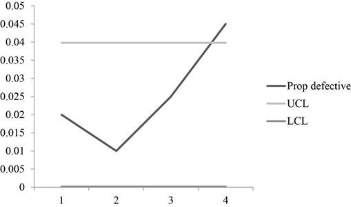
Calculation of fraction defective in each sample:
| n | 200 | |||
| Sample | 1 | 2 | 3 | 4 |
| Number with errors | 4 | 2 | 5 | 9 |
| Prop defective | 0.02 | 0.01 | 0.025 | 0.045 |
Excel Worksheet:
The proportion defective is calculated by dividing the number of errors with the number of samples. For sample 1, the number of errors 4 is divided by 200 which give 0.02 as prop defective.
Hence, the fraction defective is shown in Table 1.
b)
To determine: The estimation for fraction defective when true fraction defective for the process is unknown.
Introduction: Quality is a measure of excellence or a state of being free from deficiencies, defects and important variations. It is obtained by consistent and strict commitment to certain standards to attain uniformity of a product to satisfy consumers’ requirement.
b)
Answer to Problem 5P
Explanation of Solution
Given information:
| Sample | 1 | 2 | 3 | 4 |
| Number with errors | 4 | 2 | 5 | 9 |
Calculation of fraction defective:
The fraction defective is calculated when true fraction defective is unknown.
Total number of defective is calculated by adding the number of errors, (4+2+5+9) which accounts to 20
The fraction defective is calculated by dividing total number of defective with total number of observation which is 20 is divided with the product of 4 and 200 which is 0.025.
Hence, the fraction defective is 0.025.
c)
To determine: The estimate of mean and standard deviation of the sampling distribution of fraction defective for samples for the size.
Introduction:
Control chart:
It is a graph used to analyze the process change over a time period. A control chart has a upper control limit, and lower control which are used plot the time order.
c)
Answer to Problem 5P
Explanation of Solution
Given information:
| Sample | 1 | 2 | 3 | 4 |
| Number with errors | 4 | 2 | 5 | 9 |
Estimate of mean and standard deviation of the sampling distribution:
Mean = 0.025 (from equation (1))
The estimate for mean is shown in equation (1) and standard deviation is calculated by substituting the value which yields 0.011.
Hence, estimate of mean and standard deviation of the sampling distribution is 0.025 and 0.011.
d)
To determine: The control limits that would give an alpha risk of 0.03 for the process.
Introduction:
Control chart:
It is a graph used to analyze the process change over a time period. A control chart has a upper control limit, and lower control which are used plot the time order.
d)
Answer to Problem 5P
Explanation of Solution
Given information:
| Sample | 1 | 2 | 3 | 4 |
| Number with errors | 4 | 2 | 5 | 9 |
Control limits that would give an alpha risk of 0.03 for the process:
0.015 is in each tail and using z-factor table, value that corresponds to 0.5000 – 0.0150 is 0.4850 which is z = 2.17.
The UCL is calculated by adding 0.025 with the product of 2.17 and 0.011 which gives 0.0489 and LCL is calculated by subtracting 0.025 with the product of 2.17 and 0.011 which yields 0.0011.
Hence, the control limits that would give an alpha risk of 0.03 for the process are 0.0489 and 0.0011.
e)
To determine: The alpha risks that control limits 0.47 and 0.003 will provide.
Introduction:
Control chart:
It is a graph used to analyze the process change over a time period. A control chart has a upper control limit, and lower control which are used plot the time order.
e)
Answer to Problem 5P
Explanation of Solution
Given information:
| Sample | 1 | 2 | 3 | 4 |
| Number with errors | 4 | 2 | 5 | 9 |
Alpha risks that control limits 0.47 and 0.003 will provide:
The following equation z value can be calculated,
From z factor table, the probability value which corresponds to z = 2.00 is 0.4772, on each tail,
0.0228 is observed on each tail and doubling the value gives 0.0456 which is the alpha risk.
Hence, alpha risks that control limits 0.47 and 0.003 will provide is 0.0456
f)
To determine: Whether the process is in control when using 0.047 and 0.003.
Introduction:
Control chart:
It is a graph used to analyze the process change over a time period. A control chart has an upper control limit, and lower control which are used plot the time order.
f)
Answer to Problem 5P
Explanation of Solution
Given information:
| Sample | 1 | 2 | 3 | 4 |
| Number with errors | 4 | 2 | 5 | 9 |
Calculation of fraction defective in each sample:
| n | 200 | |||
| Sample | 1 | 2 | 3 | 4 |
| Number with errors | 4 | 2 | 5 | 9 |
| Prop defective | 0.02 | 0.01 | 0.025 | 0.045 |
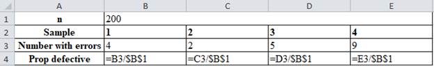
UCL = 0.047 & LCL = 0.003
Graph:
A graph is plotted using UCL, LCL and prop defective values which show that all the sample points are well within the control limits which makes the process to be in control.
Hence, the process is within control for the limits 0.047 & 0.003.
g)
To determine: The mean and standard deviation of the sampling distribution.
Introduction:
Control chart:
It is a graph used to analyze the process change over a time period. A control chart has a upper control limit, and lower control which are used plot the time order.
g)
Answer to Problem 5P
Explanation of Solution
Given information:
| Sample | 1 | 2 | 3 | 4 |
| Number with errors | 4 | 2 | 5 | 9 |
Long run fraction defective of the process is 0.02
Calculation of mean and standard deviation of the sampling distribution:
Fraction defective in each sample:
| n | 200 | |||
| Sample | 1 | 2 | 3 | 4 |
| Number with errors | 4 | 2 | 5 | 9 |
| Prop defective | 0.02 | 0.01 | 0.025 | 0.045 |
The mean is calculated by taking average for the proportion defective,
The values of the proportion defective are added and divided by 4 which give 0.02.
The standard deviation is calculated using the formula,
The standard deviation is calculated by substituting the values in the above formula and taking square root for the resultant value which yields 0.099.
Hence, mean and standard deviation of the sampling distribution is 0.02&0.0099.
h)
To construct: A control chart using two sigma control limits and check whether the process is in control.
Introduction:
Control chart:
It is a graph used to analyze the process change over a time period. A control chart has a upper control limit, and lower control which are used plot the time order.
h)
Answer to Problem 5P
Explanation of Solution
Given information:
| Sample | 1 | 2 | 3 | 4 |
| Number with errors | 4 | 2 | 5 | 9 |
Fraction defective in each sample:
| n | 200 | |||
| Sample | 1 | 2 | 3 | 4 |
| Number with errors | 4 | 2 | 5 | 9 |
| Prop defective | 0.02 | 0.01 | 0.025 | 0.045 |
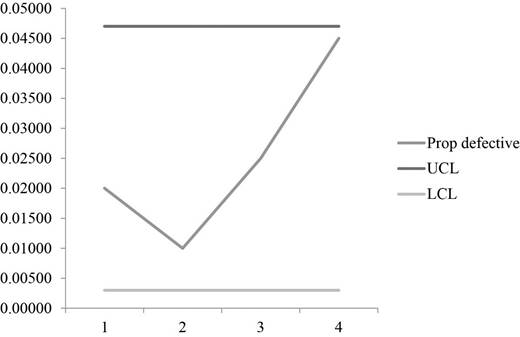
Calculation of control limits:
The control limits are calculated using the above formula and substituting the values and taking square root gives the control limits of the UCL and LCL which are 0.0398 and 0.0002 respectively.
Graph:
A graph is plotted using the fraction defective, UCL and LCL values which shows that one sample points is beyond the control region which makes the process to be out of control.
Hence, control chart is constructed using two-sigma control limits and the chart shows that the process is not in control.
Want to see more full solutions like this?
Chapter 10 Solutions
Operations Management


- At Quick Car Wash, the wash process is advertised to take less than 6 minutes. Consequently, management has set a target average of 330 seconds for the wash process. Suppose the average range for a sample of 7 cars is 10 seconds. Use the accompanying table to establish control limits for sample means and ranges for the car wash process. Click the icon to view the table of factors for calculating three-sigma limits for the x-chart and R-chart. The UCLR equals seconds and the LCLR equals seconds. (Enter your responses rounded to two decimal places.)arrow_forwardIf Jeremy who is the VP for the operations, proceeds with their existing prototype (which is option a), the firm can then expect sales to be 120,000 units at $550 each. And with a probability of 0.52 and a 0.48 probability of 65,000 at $550. we However, he uses his value analysis team (option b), the firm expects sales of 75,000 units at $770, with a probability of 0.78 and a 0.22 probability of 65,000 units at $770. Value engineering, at a cost of $100,000, is only used in option b. Which option for this has the highest expected monetary value (EMV)? The EMV for option a is $? The EMV for option b is $? Which has the highest expected monetary value. A or B?arrow_forwardPart 1 of 2 Jim's Outfitters, Inc., makes custom western shirts. The shirts could be flawed in various ways, including flaws in the weave or color of the fabric, loose buttons or decorations, wrong dimensions, and uneven stitches. Jim randomly examined 10 shirts, with the following results shown to the right. Shirt Defects 1 7 2 1 4 13 3 10 2 8 5 9 10 8 7 a. Assuming that 10 observations are adequate for these purposes, determine the three-sigma control limits for defects per shirt. The UCLC equals and the LCL equals (Enter your responses rounded to two decimal places. If your answer for LCL is negative, enter this value as 0.)arrow_forward
- Management at Webster Chemical Company is concerned as to whether caulking tubes are being properly capped. If a significant proportion of the tubes are not being sealed, Webster is placing its customers in a messy situation. Tubes are packaged in large boxes of 144. Several boxes are inspected, and the following numbers of leaking tubes are found: Sample Tubes Sample Tubes Sample Tubes 1 7 8 7 15 7 2 7 9 8 16 9 3 6 10 7 17 3 4 4 11 1 18 7 5 8 12 8 19 7 6 7 2 9 13 14 1 20 6 7 Total 121 Calculate p-chart three-sigma control limits to assess whether the capping process is in statistical control. The UCLp equals and the LCLp equals (Enter your responses rounded to three decimal places. If your answer for LCLp is negative, enter this value as 0.)arrow_forwardAspen Plastics produces plastic bottles to customer order. The quality inspector randomly selects four bottles from the bottle machine and measures the outside diameter of the bottle neck, a critical quality dimension that determines whether the bottle cap will fit properly. The dimensions (in.) from the last six samples are Bottle Sample 1 2 3 4 1 0.624 0.586 0.602 0.591 2 0.613 0.599 0.578 0.618 3 0.606 0.585 0.587 0.623 4 0.581 0.623 0.571 0.610 5 0.609 0.610 0.623 0.617 6 0.605 0.573 0.570 0.602 Click the icon to view the table of factors for calculating three-sigma limits for the x-chart and R-chart. Suppose that the specification for the bottle neck diameter is 0.600 ± 0.050 in. and the population standard deviation is 0.014 in. a. What is the process capability index? The Cpk is (Enter your response rounded to two decimal places.)arrow_forwardHow would you handle the Apple 'batterygate' scandal as an operations manager? What quality measures would you take to fix the problem and prevent it from happening again? When would you implement these measures and communicate with the stakeholders?arrow_forward
- Perosnal Thoughts about the articlearrow_forwardRevenue retrieval for Brew Mini= $ round response to two decimal places What would be the best design alternative? Brew master or brew miniarrow_forwardThe revenue retrieval for PG Glass design is ?. Enter response as a whole number). The revenue retrieval for Glass Unlimited design is ? (enter your response as a whole number). What is The best design alternative? Glass unlimited or PG Glass?arrow_forward
 Practical Management ScienceOperations ManagementISBN:9781337406659Author:WINSTON, Wayne L.Publisher:Cengage,