Essentials of Business Analytics (MindTap Course List)
2nd Edition
ISBN: 9781305627734
Author: Jeffrey D. Camm, James J. Cochran, Michael J. Fry, Jeffrey W. Ohlmann, David R. Anderson
Publisher: Cengage Learning
expand_more
expand_more
format_list_bulleted
Videos
Textbook Question
Chapter 8, Problem 24P
The quarterly sales data (number of copies sold) for a college textbook over the past three years are as follows:
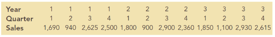
- a. Construct a time series plot. What type of pattern exists in the data?
- b. Use a regression model with dummy variables as follows to develop an equation to account for seasonal effects in the data: Qtr1 = l if quarter l, 0 otherwise; Qtr2 = l if quarter 2, 0 otherwise; Qtr3 = 1 if quarter 3, 0 otherwise.
- c. Based on the model you developed in part (b), compute the quarterly forecasts for next year.
- d. Let t = 1 to refer to the observation in quarter 1 of year 1; t = 2 to refer to the observation in quarter 2 of year 1; …; and t = 12 to refer to the observation in quarter 4 of year 3. Using the dummy variables defined in part (b) and t, develop an equation to account for seasonal effects and any linear trend in the time series.
- e. Based upon the seasonal effects in the data and linear trend, compute the quarterly forecasts for next year.
- f. Is the model you developed in part (b) or the model you developed in part (d) more effective? Justify your answer.
Expert Solution & Answer
Want to see the full answer?
Check out a sample textbook solution
Students have asked these similar questions
Need help with the following statistic problems.
Need help with the following questions on statistics.
Need help with these following statistic questions.
Chapter 8 Solutions
Essentials of Business Analytics (MindTap Course List)
Ch. 8 - Consider the following time series data:
Using...Ch. 8 - Refer to the time series data in Problem 1. Using...Ch. 8 - Problems 1 and 2 used different forecasting...Ch. 8 - Consider the following time series data:
Compute...Ch. 8 - Consider the following time series...Ch. 8 - Consider the following time series...Ch. 8 - Refer to the gasoline sales time series data in...Ch. 8 - Prob. 8PCh. 8 - Prob. 9PCh. 8 - Prob. 10P
Ch. 8 - For the Hawkins Company, the monthly percentages...Ch. 8 - Corporate triple A bond interest rates for 12...Ch. 8 - The values of Alabama building contracts (in...Ch. 8 - The following time series shows the sales of a...Ch. 8 - Prob. 15PCh. 8 - The following table reports the percentage of...Ch. 8 - Consider the following time series: a. Construct a...Ch. 8 - Consider the following time series:
Construct a...Ch. 8 - Because of high tuition costs at state and private...Ch. 8 - The Seneca Children’s Fund (SCF) is a local...Ch. 8 - The president of a small manufacturing firm is...Ch. 8 - Consider the following time series: a. Construct a...Ch. 8 - Consider the following time series...Ch. 8 - The quarterly sales data (number of copies sold)...Ch. 8 - Prob. 25PCh. 8 - South Shore Construction builds permanent docks...Ch. 8 - Hogs & Dawgs is an ice cream parlor on the border...Ch. 8 - Donna Nickles manages a gasoline station on the...Ch. 8 - The Vintage Restaurant, on Captiva Island near...
Knowledge Booster


Learn more about
Need a deep-dive on the concept behind this application? Look no further. Learn more about this topic, statistics and related others by exploring similar questions and additional content below.Similar questions
- 2PM Tue Mar 4 7 Dashboard Calendar To Do Notifications Inbox File Details a 25/SP-CIT-105-02 Statics for Technicians Q-7 Determine the resultant of the load system shown. Locate where the resultant intersects grade with respect to point A at the base of the structure. 40 N/m 2 m 1.5 m 50 N 100 N/m Fig.- Problem-7 4 m Gradearrow_forwardNsjsjsjarrow_forwardA smallish urn contains 16 small plastic bunnies - 9 of which are pink and 7 of which are white. 10 bunnies are drawn from the urn at random with replacement, and X is the number of pink bunnies that are drawn. (a) P(X=6)[Select] (b) P(X>7) ≈ [Select]arrow_forward
- A smallish urn contains 25 small plastic bunnies - 7 of which are pink and 18 of which are white. 10 bunnies are drawn from the urn at random with replacement, and X is the number of pink bunnies that are drawn. (a) P(X = 5)=[Select] (b) P(X<6) [Select]arrow_forwardElementary StatisticsBase on the same given data uploaded in module 4, will you conclude that the number of bathroom of houses is a significant factor for house sellprice? I your answer is affirmative, you need to explain how the number of bathroom influences the house price, using a post hoc procedure. (Please treat number of bathrooms as a categorical variable in this analysis)Base on the same given data, conduct an analysis for the variable sellprice to see if sale price is influenced by living area. Summarize your finding including all regular steps (learned in this module) for your method. Also, will you conclude that larger house corresponding to higher price (justify)?Each question need to include a spss or sas output. Instructions: You have to use SAS or SPSS to perform appropriate procedure: ANOVA or Regression based on the project data (provided in the module 4) and research question in the project file. Attach the computer output of all key steps (number) quoted in…arrow_forwardElementary StatsBase on the given data uploaded in module 4, change the variable sale price into two categories: abovethe mean price or not; and change the living area into two categories: above the median living area ornot ( your two group should have close number of houses in each group). Using the resulting variables,will you conclude that larger house corresponding to higher price?Note: Need computer output, Ho and Ha, P and decision. If p is small, you need to explain what type ofdependency (association) we have using an appropriate pair of percentages. Please include how to use the data in SPSS and interpretation of data.arrow_forward
- An environmental research team is studying the daily rainfall (in millimeters) in a region over 100 days. The data is grouped into the following histogram bins: Rainfall Range (mm) Frequency 0-9.9 15 10 19.9 25 20-29.9 30 30-39.9 20 ||40-49.9 10 a) If a random day is selected, what is the probability that the rainfall was at least 20 mm but less than 40 mm? b) Estimate the mean daily rainfall, assuming the rainfall in each bin is uniformly distributed and the midpoint of each bin represents the average rainfall for that range. c) Construct the cumulative frequency distribution and determine the rainfall level below which 75% of the days fall. d) Calculate the estimated variance and standard deviation of the daily rainfall based on the histogram data.arrow_forwardAn electronics company manufactures batches of n circuit boards. Before a batch is approved for shipment, m boards are randomly selected from the batch and tested. The batch is rejected if more than d boards in the sample are found to be faulty. a) A batch actually contains six faulty circuit boards. Find the probability that the batch is rejected when n = 20, m = 5, and d = 1. b) A batch actually contains nine faulty circuit boards. Find the probability that the batch is rejected when n = 30, m = 10, and d = 1.arrow_forwardTwenty-eight applicants interested in working for the Food Stamp program took an examination designed to measure their aptitude for social work. A stem-and-leaf plot of the 28 scores appears below, where the first column is the count per branch, the second column is the stem value, and the remaining digits are the leaves. a) List all the values. Count 1 Stems Leaves 4 6 1 4 6 567 9 3688 026799 9 8 145667788 7 9 1234788 b) Calculate the first quartile (Q1) and the third Quartile (Q3). c) Calculate the interquartile range. d) Construct a boxplot for this data.arrow_forward
- Pam, Rob and Sam get a cake that is one-third chocolate, one-third vanilla, and one-third strawberry as shown below. They wish to fairly divide the cake using the lone chooser method. Pam likes strawberry twice as much as chocolate or vanilla. Rob only likes chocolate. Sam, the chooser, likes vanilla and strawberry twice as much as chocolate. In the first division, Pam cuts the strawberry piece off and lets Rob choose his favorite piece. Based on that, Rob chooses the chocolate and vanilla parts. Note: All cuts made to the cake shown below are vertical.Which is a second division that Rob would make of his share of the cake?arrow_forwardThree players (one divider and two choosers) are going to divide a cake fairly using the lone divider method. The divider cuts the cake into three slices (s1, s2, and s3). If the choosers' declarations are Chooser 1: {s1 , s2} and Chooser 2: {s2 , s3}. Using the lone-divider method, how many different fair divisions of this cake are possible?arrow_forwardTheorem 2.6 (The Minkowski inequality) Let p≥1. Suppose that X and Y are random variables, such that E|X|P <∞ and E|Y P <00. Then X+YpX+Yparrow_forward
arrow_back_ios
SEE MORE QUESTIONS
arrow_forward_ios
Recommended textbooks for you
 Functions and Change: A Modeling Approach to Coll...AlgebraISBN:9781337111348Author:Bruce Crauder, Benny Evans, Alan NoellPublisher:Cengage Learning
 Holt Mcdougal Larson Pre-algebra: Student Edition...AlgebraISBN:9780547587776Author:HOLT MCDOUGALPublisher:HOLT MCDOUGAL
 Glencoe Algebra 1, Student Edition, 9780079039897...AlgebraISBN:9780079039897Author:CarterPublisher:McGraw Hill
 Trigonometry (MindTap Course List)TrigonometryISBN:9781337278461Author:Ron LarsonPublisher:Cengage Learning
Functions and Change: A Modeling Approach to Coll...
Algebra
ISBN:9781337111348
Author:Bruce Crauder, Benny Evans, Alan Noell
Publisher:Cengage Learning
Holt Mcdougal Larson Pre-algebra: Student Edition...
Algebra
ISBN:9780547587776
Author:HOLT MCDOUGAL
Publisher:HOLT MCDOUGAL
Glencoe Algebra 1, Student Edition, 9780079039897...
Algebra
ISBN:9780079039897
Author:Carter
Publisher:McGraw Hill
Trigonometry (MindTap Course List)
Trigonometry
ISBN:9781337278461
Author:Ron Larson
Publisher:Cengage Learning
Time Series Analysis Theory & Uni-variate Forecasting Techniques; Author: Analytics University;https://www.youtube.com/watch?v=_X5q9FYLGxM;License: Standard YouTube License, CC-BY
Operations management 101: Time-series, forecasting introduction; Author: Brandoz Foltz;https://www.youtube.com/watch?v=EaqZP36ool8;License: Standard YouTube License, CC-BY