
Videos
(a)
Draw the time-series plot for the given data.
Identify the pattern.
(a)
Explanation of Solution
Step-by-step procedure to construct time-series plot is given below.
- Enter the data in columns A and B. Select the data.
- Click on Insert tab and then click on line.
- Select line with markers
The output is given below:
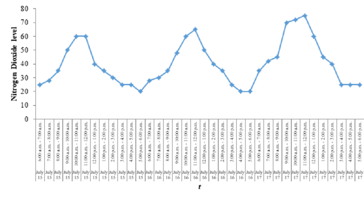
From the above time-series plot, it is clear that plot shows upward trend. Also, there exists seasonal pattern.
(b)
Find a multiple regression equation that represents seasonal effect using dummy variables for the given data.
(b)
Answer to Problem 25P
The regression equation is,
Explanation of Solution
Dummy variables are defined as given below:
Also, all the dummy variables are 0 when the reading time corresponds to 5:00 p.m. to 6:00 p.m.
The given data is entered as given below:
| Hourly Dummy Variables | |||||||||||||
| Date | Hour | yt | 1 | 2 | 3 | 4 | 5 | 6 | 7 | 8 | 9 | 10 | 11 |
| July 15 | 6:00 a.m. - 7:00 a.m. | 25 | 1 | 0 | 0 | 0 | 0 | 0 | 0 | 0 | 0 | 0 | 0 |
| July 15 | 7:00 a.m. - 8:00 a.m. | 28 | 0 | 1 | 0 | 0 | 0 | 0 | 0 | 0 | 0 | 0 | 0 |
| July 15 | 8:00 a.m. - 9:00 a.m. | 35 | 0 | 0 | 1 | 0 | 0 | 0 | 0 | 0 | 0 | 0 | 0 |
| July 15 | 9:00 a.m. - 10:00 a.m. | 50 | 0 | 0 | 0 | 1 | 0 | 0 | 0 | 0 | 0 | 0 | 0 |
| July 15 | 10:00 a.m. - 11:00 a.m. | 60 | 0 | 0 | 0 | 0 | 1 | 0 | 0 | 0 | 0 | 0 | 0 |
| July 15 | 11:00 a.m. - 12:00 p.m. | 60 | 0 | 0 | 0 | 0 | 0 | 1 | 0 | 0 | 0 | 0 | 0 |
| July 15 | 12:00 p.m. - 1:00 p.m. | 40 | 0 | 0 | 0 | 0 | 0 | 0 | 1 | 0 | 0 | 0 | 0 |
| July 15 | 1:00 p.m. - 2:00 p.m. | 35 | 0 | 0 | 0 | 0 | 0 | 0 | 0 | 1 | 0 | 0 | 0 |
| July 15 | 2:00 p.m. - 3:00 p.m. | 30 | 0 | 0 | 0 | 0 | 0 | 0 | 0 | 0 | 1 | 0 | 0 |
| July 15 | 3:00 p.m. - 4:00 p.m. | 25 | 0 | 0 | 0 | 0 | 0 | 0 | 0 | 0 | 0 | 1 | 0 |
| July 15 | 4:00 p.m. - 5:00 p.m. | 25 | 0 | 0 | 0 | 0 | 0 | 0 | 0 | 0 | 0 | 0 | 1 |
| July 15 | 5:00 p.m. - 6:00 p.m. | 20 | 0 | 0 | 0 | 0 | 0 | 0 | 0 | 0 | 0 | 0 | 0 |
| July 16 | 6:00 a.m. - 7:00 a.m. | 28 | 1 | 0 | 0 | 0 | 0 | 0 | 0 | 0 | 0 | 0 | 0 |
| July 16 | 7:00 a.m. - 8:00 a.m. | 30 | 0 | 1 | 0 | 0 | 0 | 0 | 0 | 0 | 0 | 0 | 0 |
| July 16 | 8:00 a.m. - 9:00 a.m. | 35 | 0 | 0 | 1 | 0 | 0 | 0 | 0 | 0 | 0 | 0 | 0 |
| July 16 | 9:00 a.m. - 10:00 a.m. | 48 | 0 | 0 | 0 | 1 | 0 | 0 | 0 | 0 | 0 | 0 | 0 |
| July 16 | 10:00 a.m. - 11:00 a.m. | 60 | 0 | 0 | 0 | 0 | 1 | 0 | 0 | 0 | 0 | 0 | 0 |
| July 16 | 11:00 a.m. - 12:00 p.m. | 65 | 0 | 0 | 0 | 0 | 0 | 1 | 0 | 0 | 0 | 0 | 0 |
| July 16 | 12:00 p.m. - 1:00 p.m. | 50 | 0 | 0 | 0 | 0 | 0 | 0 | 1 | 0 | 0 | 0 | 0 |
| July 16 | 1:00 p.m. - 2:00 p.m. | 40 | 0 | 0 | 0 | 0 | 0 | 0 | 0 | 1 | 0 | 0 | 0 |
| July 16 | 2:00 p.m. - 3:00 p.m. | 35 | 0 | 0 | 0 | 0 | 0 | 0 | 0 | 0 | 1 | 0 | 0 |
| July 16 | 3:00 p.m. - 4:00 p.m. | 25 | 0 | 0 | 0 | 0 | 0 | 0 | 0 | 0 | 0 | 1 | 0 |
| July 16 | 4:00 p.m. - 5:00 p.m. | 20 | 0 | 0 | 0 | 0 | 0 | 0 | 0 | 0 | 0 | 0 | 1 |
| July 16 | 5:00 p.m. - 6:00 p.m. | 20 | 0 | 0 | 0 | 0 | 0 | 0 | 0 | 0 | 0 | 0 | 0 |
| July 17 | 6:00 a.m. - 7:00 a.m. | 35 | 1 | 0 | 0 | 0 | 0 | 0 | 0 | 0 | 0 | 0 | 0 |
| July 17 | 7:00 a.m. - 8:00 a.m. | 42 | 0 | 1 | 0 | 0 | 0 | 0 | 0 | 0 | 0 | 0 | 0 |
| July 17 | 8:00 a.m. - 9:00 a.m. | 45 | 0 | 0 | 1 | 0 | 0 | 0 | 0 | 0 | 0 | 0 | 0 |
| July 17 | 9:00 a.m. - 10:00 a.m. | 70 | 0 | 0 | 0 | 1 | 0 | 0 | 0 | 0 | 0 | 0 | 0 |
| July 17 | 10:00 a.m. - 11:00 a.m. | 72 | 0 | 0 | 0 | 0 | 1 | 0 | 0 | 0 | 0 | 0 | 0 |
| July 17 | 11:00 a.m. - 12:00 p.m. | 75 | 0 | 0 | 0 | 0 | 0 | 1 | 0 | 0 | 0 | 0 | 0 |
| July 17 | 12:00 p.m. - 1:00 p.m. | 60 | 0 | 0 | 0 | 0 | 0 | 0 | 1 | 0 | 0 | 0 | 0 |
| July 17 | 1:00 p.m. - 2:00 p.m. | 45 | 0 | 0 | 0 | 0 | 0 | 0 | 0 | 1 | 0 | 0 | 0 |
| July 17 | 2:00 p.m. - 3:00 p.m. | 40 | 0 | 0 | 0 | 0 | 0 | 0 | 0 | 0 | 1 | 0 | 0 |
| July 17 | 3:00 p.m. - 4:00 p.m. | 25 | 0 | 0 | 0 | 0 | 0 | 0 | 0 | 0 | 0 | 1 | 0 |
| July 17 | 4:00 p.m. - 5:00 p.m. | 25 | 0 | 0 | 0 | 0 | 0 | 0 | 0 | 0 | 0 | 0 | 1 |
| July 17 | 5:00 p.m. - 6:00 p.m. | 25 | 0 | 0 | 0 | 0 | 0 | 0 | 0 | 0 | 0 | 0 | 0 |
Step-by-step procedure to obtain multiple linear regression line is given below.
- Enter the data in columns A to M.
- Click on Data tab and then Data Analysis.
- Select Regression and click ok.
- In Input Y
Range select, $B$2:$B$37 and Input X Range select $C$2:$M$37 - Click Ok.
The output is given below:
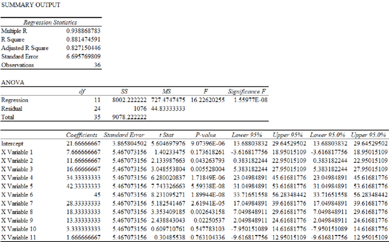
From the output the regression equation is,
Here, X Variable 1 represents Hour1, X Variable 2 represents Hour2, … X variable 11 represents Hour11.
(c)
Find the estimates of the levels of nitrogen for July 18 using the model developed in part (b).
(c)
Explanation of Solution
From part (b), the regression equation is,
Forecast for July 18 is obtained as given below:
| Hourly forecast | Calculation | |
| Hour1 | 29.34 | |
| Hour2 | 33.34 | |
| Hour3 | 38.34 | |
| Hour4 | 56 | |
| Hour5 | 64 | |
| Hour6 | 66.67 | |
| Hour7 | 50 | |
| Hour8 | 40 | |
| Hour9 | 35 | |
| Hour10 | 25 | |
| Hour11 | 23.34 | |
| Hour12 | 21.67 | 21.67 |
(d)
Construct a multiple regression equation that represents seasonal effect using dummy variables and a t variable for the given data.
(d)
Answer to Problem 25P
The regression equation is,
Explanation of Solution
Create a variable t such that t = 1 for hour 1 on July 15, t = 2 for hour 2 on July 2, …, t = 36 for hour 12 on July 18.
The given data is entered as given below:
| Hourly Dummy Variables | ||||||||||||||
| Date | Hour | yt | 1 | 2 | 3 | 4 | 5 | 6 | 7 | 8 | 9 | 10 | 11 | t |
| July 15 | 6:00 a.m. - 7:00 a.m. | 25 | 1 | 0 | 0 | 0 | 0 | 0 | 0 | 0 | 0 | 0 | 0 | 1 |
| July 15 | 7:00 a.m. - 8:00 a.m. | 28 | 0 | 1 | 0 | 0 | 0 | 0 | 0 | 0 | 0 | 0 | 0 | 2 |
| July 15 | 8:00 a.m. - 9:00 a.m. | 35 | 0 | 0 | 1 | 0 | 0 | 0 | 0 | 0 | 0 | 0 | 0 | 3 |
| July 15 | 9:00 a.m. - 10:00 a.m. | 50 | 0 | 0 | 0 | 1 | 0 | 0 | 0 | 0 | 0 | 0 | 0 | 4 |
| July 15 | 10:00 a.m. - 11:00 a.m. | 60 | 0 | 0 | 0 | 0 | 1 | 0 | 0 | 0 | 0 | 0 | 0 | 5 |
| July 15 | 11:00 a.m. - 12:00 p.m. | 60 | 0 | 0 | 0 | 0 | 0 | 1 | 0 | 0 | 0 | 0 | 0 | 6 |
| July 15 | 12:00 p.m. - 1:00 p.m. | 40 | 0 | 0 | 0 | 0 | 0 | 0 | 1 | 0 | 0 | 0 | 0 | 7 |
| July 15 | 1:00 p.m. - 2:00 p.m. | 35 | 0 | 0 | 0 | 0 | 0 | 0 | 0 | 1 | 0 | 0 | 0 | 8 |
| July 15 | 2:00 p.m. - 3:00 p.m. | 30 | 0 | 0 | 0 | 0 | 0 | 0 | 0 | 0 | 1 | 0 | 0 | 9 |
| July 15 | 3:00 p.m. - 4:00 p.m. | 25 | 0 | 0 | 0 | 0 | 0 | 0 | 0 | 0 | 0 | 1 | 0 | 10 |
| July 15 | 4:00 p.m. - 5:00 p.m. | 25 | 0 | 0 | 0 | 0 | 0 | 0 | 0 | 0 | 0 | 0 | 1 | 11 |
| July 15 | 5:00 p.m. - 6:00 p.m. | 20 | 0 | 0 | 0 | 0 | 0 | 0 | 0 | 0 | 0 | 0 | 0 | 12 |
| July 16 | 6:00 a.m. - 7:00 a.m. | 28 | 1 | 0 | 0 | 0 | 0 | 0 | 0 | 0 | 0 | 0 | 0 | 13 |
| July 16 | 7:00 a.m. - 8:00 a.m. | 30 | 0 | 1 | 0 | 0 | 0 | 0 | 0 | 0 | 0 | 0 | 0 | 14 |
| July 16 | 8:00 a.m. - 9:00 a.m. | 35 | 0 | 0 | 1 | 0 | 0 | 0 | 0 | 0 | 0 | 0 | 0 | 15 |
| July 16 | 9:00 a.m. - 10:00 a.m. | 48 | 0 | 0 | 0 | 1 | 0 | 0 | 0 | 0 | 0 | 0 | 0 | 16 |
| July 16 | 10:00 a.m. - 11:00 a.m. | 60 | 0 | 0 | 0 | 0 | 1 | 0 | 0 | 0 | 0 | 0 | 0 | 17 |
| July 16 | 11:00 a.m. - 12:00 p.m. | 65 | 0 | 0 | 0 | 0 | 0 | 1 | 0 | 0 | 0 | 0 | 0 | 18 |
| July 16 | 12:00 p.m. - 1:00 p.m. | 50 | 0 | 0 | 0 | 0 | 0 | 0 | 1 | 0 | 0 | 0 | 0 | 19 |
| July 16 | 1:00 p.m. - 2:00 p.m. | 40 | 0 | 0 | 0 | 0 | 0 | 0 | 0 | 1 | 0 | 0 | 0 | 20 |
| July 16 | 2:00 p.m. - 3:00 p.m. | 35 | 0 | 0 | 0 | 0 | 0 | 0 | 0 | 0 | 1 | 0 | 0 | 21 |
| July 16 | 3:00 p.m. - 4:00 p.m. | 25 | 0 | 0 | 0 | 0 | 0 | 0 | 0 | 0 | 0 | 1 | 0 | 22 |
| July 16 | 4:00 p.m. - 5:00 p.m. | 20 | 0 | 0 | 0 | 0 | 0 | 0 | 0 | 0 | 0 | 0 | 1 | 23 |
| July 16 | 5:00 p.m. - 6:00 p.m. | 20 | 0 | 0 | 0 | 0 | 0 | 0 | 0 | 0 | 0 | 0 | 0 | 24 |
| July 17 | 6:00 a.m. - 7:00 a.m. | 35 | 1 | 0 | 0 | 0 | 0 | 0 | 0 | 0 | 0 | 0 | 0 | 25 |
| July 17 | 7:00 a.m. - 8:00 a.m. | 42 | 0 | 1 | 0 | 0 | 0 | 0 | 0 | 0 | 0 | 0 | 0 | 26 |
| July 17 | 8:00 a.m. - 9:00 a.m. | 45 | 0 | 0 | 1 | 0 | 0 | 0 | 0 | 0 | 0 | 0 | 0 | 27 |
| July 17 | 9:00 a.m. - 10:00 a.m. | 70 | 0 | 0 | 0 | 1 | 0 | 0 | 0 | 0 | 0 | 0 | 0 | 28 |
| July 17 | 10:00 a.m. - 11:00 a.m. | 72 | 0 | 0 | 0 | 0 | 1 | 0 | 0 | 0 | 0 | 0 | 0 | 29 |
| July 17 | 11:00 a.m. - 12:00 p.m. | 75 | 0 | 0 | 0 | 0 | 0 | 1 | 0 | 0 | 0 | 0 | 0 | 30 |
| July 17 | 12:00 p.m. - 1:00 p.m. | 60 | 0 | 0 | 0 | 0 | 0 | 0 | 1 | 0 | 0 | 0 | 0 | 31 |
| July 17 | 1:00 p.m. - 2:00 p.m. | 45 | 0 | 0 | 0 | 0 | 0 | 0 | 0 | 1 | 0 | 0 | 0 | 32 |
| July 17 | 2:00 p.m. - 3:00 p.m. | 40 | 0 | 0 | 0 | 0 | 0 | 0 | 0 | 0 | 1 | 0 | 0 | 33 |
| July 17 | 3:00 p.m. - 4:00 p.m. | 25 | 0 | 0 | 0 | 0 | 0 | 0 | 0 | 0 | 0 | 1 | 0 | 34 |
| July 17 | 4:00 p.m. - 5:00 p.m. | 25 | 0 | 0 | 0 | 0 | 0 | 0 | 0 | 0 | 0 | 0 | 1 | 35 |
| July 17 | 5:00 p.m. - 6:00 p.m. | 25 | 0 | 0 | 0 | 0 | 0 | 0 | 0 | 0 | 0 | 0 | 0 | 36 |
Step-by-step procedure to obtain multiple linear regression line is given below.
- Enter the data in columns A to N.
- Click on Data tab and then Data Analysis.
- Select Regression and click ok.
- In Input Y Range select, $B$2:$B$37 and Input X Range select $C$2:$N$37
- Click Ok.
The output is given below:
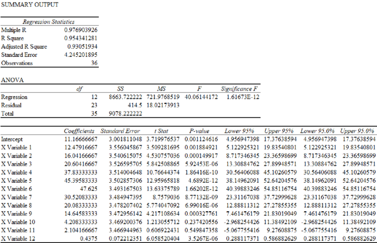
From the output the regression equation is,
Here, X Variable 1 represents Hour1, X Variable 2 represents Hour2,… X variable 11 represents Hour11 and X variable 12 represents t.
(e)
Calculate the estimates of the levels of nitrogen for July 18 using the model developed in part (d).
(e)
Explanation of Solution
From part (d), the regression equation is,
Forecast for July 18 is given below:
| Hourly forecast | T | Calculation | |
| 1 | 37 | 39.93 | |
| 2 | 38 | 43.93 | |
| 3 | 39 | 48.93 | |
| 4 | 40 | 66.6 | |
| 5 | 41 | 74.71 | |
| 6 | 42 | 77.28 | |
| 7 | 43 | 60.61 | |
| 8 | 44 | 50.61 | |
| 9 | 45 | 45.62 | |
| 10 | 46 | 35.62 | |
| 11 | 47 | 33.95 | |
| 12 | 48 | 32.29 |
(f)
Justify which of the models (b) or (d) is effective.
(f)
Answer to Problem 25P
Model (d) is preferred.
Explanation of Solution
For the multiple regression equation developed in part (b), MSE is obtained as given below:
| Date | Hour | yt | Forecast | Forecast Error | Squared Forecast Error |
| 15-Jul | 6:00 a.m. - 7:00 a.m. | 25 | 29.34 | -4.34 | 18.8356 |
| 15-Jul | 7:00 a.m. - 8:00 a.m. | 28 | 33.34 | -5.34 | 28.5156 |
| 15-Jul | 8:00 a.m. - 9:00 a.m. | 35 | 38.34 | -3.34 | 11.1556 |
| 15-Jul | 9:00 a.m. - 10:00 a.m. | 50 | 56 | -6 | 36 |
| 15-Jul | 10:00 a.m. - 11:00 a.m. | 60 | 64 | -4 | 16 |
| 15-Jul | 11:00 a.m. - 12:00 p.m. | 60 | 66.67 | -6.67 | 44.4889 |
| 15-Jul | 12:00 p.m. - 1:00 p.m. | 40 | 50 | -10 | 100 |
| 15-Jul | 1:00 p.m. - 2:00 p.m. | 35 | 40 | -5 | 25 |
| 15-Jul | 2:00 p.m. - 3:00 p.m. | 30 | 35 | -5 | 25 |
| 15-Jul | 3:00 p.m. - 4:00 p.m. | 25 | 25 | 0 | 0 |
| 15-Jul | 4:00 p.m. - 5:00 p.m. | 25 | 23.34 | 1.66 | 2.7556 |
| 15-Jul | 5:00 p.m. - 6:00 p.m. | 20 | 21.67 | -1.67 | 2.7889 |
| 16-Jul | 6:00 a.m. - 7:00 a.m. | 28 | 29.34 | -1.34 | 1.7956 |
| 16-Jul | 7:00 a.m. - 8:00 a.m. | 30 | 33.34 | -3.34 | 11.1556 |
| 16-Jul | 8:00 a.m. - 9:00 a.m. | 35 | 38.34 | -3.34 | 11.1556 |
| 16-Jul | 9:00 a.m. - 10:00 a.m. | 48 | 56 | -8 | 64 |
| 16-Jul | 10:00 a.m. - 11:00 a.m. | 60 | 64 | -4 | 16 |
| 16-Jul | 11:00 a.m. - 12:00 p.m. | 65 | 66.67 | -1.67 | 2.7889 |
| 16-Jul | 12:00 p.m. - 1:00 p.m. | 50 | 50 | 0 | 0 |
| 16-Jul | 1:00 p.m. - 2:00 p.m. | 40 | 40 | 0 | 0 |
| 16-Jul | 2:00 p.m. - 3:00 p.m. | 35 | 35 | 0 | 0 |
| 16-Jul | 3:00 p.m. - 4:00 p.m. | 25 | 25 | 0 | 0 |
| 16-Jul | 4:00 p.m. - 5:00 p.m. | 20 | 23.34 | -3.34 | 11.1556 |
| 16-Jul | 5:00 p.m. - 6:00 p.m. | 20 | 21.67 | -1.67 | 2.7889 |
| 17-Jul | 6:00 a.m. - 7:00 a.m. | 35 | 29.34 | 5.66 | 32.0356 |
| 17-Jul | 7:00 a.m. - 8:00 a.m. | 42 | 33.34 | 8.66 | 74.9956 |
| 17-Jul | 8:00 a.m. - 9:00 a.m. | 45 | 38.34 | 6.66 | 44.3556 |
| 17-Jul | 9:00 a.m. - 10:00 a.m. | 70 | 56 | 14 | 196 |
| 17-Jul | 10:00 a.m. - 11:00 a.m. | 72 | 64 | 8 | 64 |
| 17-Jul | 11:00 a.m. - 12:00 p.m. | 75 | 66.67 | 8.33 | 69.3889 |
| 17-Jul | 12:00 p.m. - 1:00 p.m. | 60 | 50 | 10 | 100 |
| 17-Jul | 1:00 p.m. - 2:00 p.m. | 45 | 40 | 5 | 25 |
| 17-Jul | 2:00 p.m. - 3:00 p.m. | 40 | 35 | 5 | 25 |
| 17-Jul | 3:00 p.m. - 4:00 p.m. | 25 | 25 | 0 | 0 |
| 17-Jul | 4:00 p.m. - 5:00 p.m. | 25 | 23.34 | 1.66 | 2.7556 |
| 17-Jul | 5:00 p.m. - 6:00 p.m. | 25 | 21.67 | 3.33 | 11.0889 |
| 1076.001 |
For the multiple regression equation developed in part (d), MSE is obtained as given below:
| Date | Hour | t | yt | Forecast | Forecast Error | Squared Forecast Error |
| 15-Jul | 6:00 a.m. - 7:00 a.m. | 1 | 25 | 24.09 | 0.91 | 0.8281 |
| 15-Jul | 7:00 a.m. - 8:00 a.m. | 2 | 28 | 28.09 | -0.09 | 0.0081 |
| 15-Jul | 8:00 a.m. - 9:00 a.m. | 3 | 35 | 33.09 | 1.91 | 3.6481 |
| 15-Jul | 9:00 a.m. - 10:00 a.m. | 4 | 50 | 50.76 | -0.76 | 0.5776 |
| 15-Jul | 10:00 a.m. - 11:00 a.m. | 5 | 60 | 58.87 | 1.13 | 1.2769 |
| 15-Jul | 11:00 a.m. - 12:00 p.m. | 6 | 60 | 61.44 | -1.44 | 2.0736 |
| 15-Jul | 12:00 p.m. - 1:00 p.m. | 7 | 40 | 44.77 | -4.77 | 22.7529 |
| 15-Jul | 1:00 p.m. - 2:00 p.m. | 8 | 35 | 34.77 | 0.23 | 0.0529 |
| 15-Jul | 2:00 p.m. - 3:00 p.m. | 9 | 30 | 29.78 | 0.22 | 0.0484 |
| 15-Jul | 3:00 p.m. - 4:00 p.m. | 10 | 25 | 19.78 | 5.22 | 27.2484 |
| 15-Jul | 4:00 p.m. - 5:00 p.m. | 11 | 25 | 18.11 | 6.89 | 47.4721 |
| 15-Jul | 5:00 p.m. - 6:00 p.m. | 12 | 20 | 16.45 | 3.55 | 12.6025 |
| 16-Jul | 6:00 a.m. - 7:00 a.m. | 13 | 28 | 29.37 | -1.37 | 1.8769 |
| 16-Jul | 7:00 a.m. - 8:00 a.m. | 14 | 30 | 33.37 | -3.37 | 11.3569 |
| 16-Jul | 8:00 a.m. - 9:00 a.m. | 15 | 35 | 38.37 | -3.37 | 11.3569 |
| 16-Jul | 9:00 a.m. - 10:00 a.m. | 16 | 48 | 56.04 | -8.04 | 64.6416 |
| 16-Jul | 10:00 a.m. - 11:00 a.m. | 17 | 60 | 64.15 | -4.15 | 17.2225 |
| 16-Jul | 11:00 a.m. - 12:00 p.m. | 18 | 65 | 66.72 | -1.72 | 2.9584 |
| 16-Jul | 12:00 p.m. - 1:00 p.m. | 19 | 50 | 50.05 | -0.05 | 0.0025 |
| 16-Jul | 1:00 p.m. - 2:00 p.m. | 20 | 40 | 40.05 | -0.05 | 0.0025 |
| 16-Jul | 2:00 p.m. - 3:00 p.m. | 21 | 35 | 35.06 | -0.06 | 0.0036 |
| 16-Jul | 3:00 p.m. - 4:00 p.m. | 22 | 25 | 25.06 | -0.06 | 0.0036 |
| 16-Jul | 4:00 p.m. - 5:00 p.m. | 23 | 20 | 23.39 | -3.39 | 11.4921 |
| 16-Jul | 5:00 p.m. - 6:00 p.m. | 24 | 20 | 21.73 | -1.73 | 2.9929 |
| 17-Jul | 6:00 a.m. - 7:00 a.m. | 25 | 35 | 34.65 | 0.35 | 0.1225 |
| 17-Jul | 7:00 a.m. - 8:00 a.m. | 26 | 42 | 38.65 | 3.35 | 11.2225 |
| 17-Jul | 8:00 a.m. - 9:00 a.m. | 27 | 45 | 43.65 | 1.35 | 1.8225 |
| 17-Jul | 9:00 a.m. - 10:00 a.m. | 28 | 70 | 61.32 | 8.68 | 75.3424 |
| 17-Jul | 10:00 a.m. - 11:00 a.m. | 29 | 72 | 69.43 | 2.57 | 6.6049 |
| 17-Jul | 11:00 a.m. - 12:00 p.m. | 30 | 75 | 72 | 3 | 9 |
| 17-Jul | 12:00 p.m. - 1:00 p.m. | 31 | 60 | 55.33 | 4.67 | 21.8089 |
| 17-Jul | 1:00 p.m. - 2:00 p.m. | 32 | 45 | 45.33 | -0.33 | 0.1089 |
| 17-Jul | 2:00 p.m. - 3:00 p.m. | 33 | 40 | 40.34 | -0.34 | 0.1156 |
| 17-Jul | 3:00 p.m. - 4:00 p.m. | 34 | 25 | 30.34 | -5.34 | 28.5156 |
| 17-Jul | 4:00 p.m. - 5:00 p.m. | 35 | 25 | 28.67 | -3.67 | 13.4689 |
| 17-Jul | 5:00 p.m. - 6:00 p.m. | 36 | 25 | 27.01 | -2.01 | 4.0401 |
| 414.6728 |
MSE for model in (d) is smaller than MSE for the model in (b). Thus, model (d) is preferred.
Want to see more full solutions like this?
Chapter 8 Solutions
Essentials of Business Analytics (MindTap Course List)


- Should you be confident in applying your regression equation to estimate the heart rate of a python at 35°C? Why or why not?arrow_forwardGiven your fitted regression line, what would be the residual for snake #5 (10 C)?arrow_forwardCalculate the 95% confidence interval around your estimate of r using Fisher’s z-transformation. In your final answer, make sure to back-transform to the original units.arrow_forward
- BUSINESS DISCUSSarrow_forwardA researcher wishes to estimate, with 90% confidence, the population proportion of adults who support labeling legislation for genetically modified organisms (GMOs). Her estimate must be accurate within 4% of the true proportion. (a) No preliminary estimate is available. Find the minimum sample size needed. (b) Find the minimum sample size needed, using a prior study that found that 65% of the respondents said they support labeling legislation for GMOs. (c) Compare the results from parts (a) and (b). ... (a) What is the minimum sample size needed assuming that no prior information is available? n = (Round up to the nearest whole number as needed.)arrow_forwardThe table available below shows the costs per mile (in cents) for a sample of automobiles. At a = 0.05, can you conclude that at least one mean cost per mile is different from the others? Click on the icon to view the data table. Let Hss, HMS, HLS, Hsuv and Hмy represent the mean costs per mile for small sedans, medium sedans, large sedans, SUV 4WDs, and minivans respectively. What are the hypotheses for this test? OA. Ho: Not all the means are equal. Ha Hss HMS HLS HSUV HMV B. Ho Hss HMS HLS HSUV = μMV Ha: Hss *HMS *HLS*HSUV * HMV C. Ho Hss HMS HLS HSUV =μMV = = H: Not all the means are equal. D. Ho Hss HMS HLS HSUV HMV Ha Hss HMS HLS =HSUV = HMVarrow_forward
 Glencoe Algebra 1, Student Edition, 9780079039897...AlgebraISBN:9780079039897Author:CarterPublisher:McGraw Hill
 Holt Mcdougal Larson Pre-algebra: Student Edition...AlgebraISBN:9780547587776Author:HOLT MCDOUGALPublisher:HOLT MCDOUGAL
 Trigonometry (MindTap Course List)TrigonometryISBN:9781305652224Author:Charles P. McKeague, Mark D. TurnerPublisher:Cengage Learning
 Intermediate AlgebraAlgebraISBN:9781285195728Author:Jerome E. Kaufmann, Karen L. SchwittersPublisher:Cengage Learning
 Big Ideas Math A Bridge To Success Algebra 1: Stu...AlgebraISBN:9781680331141Author:HOUGHTON MIFFLIN HARCOURTPublisher:Houghton Mifflin Harcourt
 Algebra for College StudentsAlgebraISBN:9781285195780Author:Jerome E. Kaufmann, Karen L. SchwittersPublisher:Cengage Learning