
Videos
Use exponential smoothing with a smoothing constant of 0.3 to
a) What is the MAD?
b) What is the MSE?
a)
To determine: Forecast the registrations at the seminar using exponential smoothing and hence compute MAD.
Introduction: Forecasting is used to predict future changes or demand patterns. It involves different approaches and varies with different time periods. Exponential Smoothing and Naïve forecasting methods are two of the time series methods of forecasting which use past data to forecast the future.
Answer to Problem 11P
Using exponential smoothing, the registrations at the seminar are forecasted and the computed MAD is 2.44.
Explanation of Solution
Given information:
| Year | Registrations (000) |
| 1 | 4 |
| 2 | 6 |
| 3 | 4 |
| 4 | 5 |
| 5 | 10 |
| 6 | 8 |
| 7 | 7 |
| 8 | 9 |
| 9 | 12 |
| 10 | 14 |
| 11 | 15 |
Formula to calculate the forecasted demand
Where,
Calculation to forecast demand using exponential smoothing:
| Year | Registrations (000) | Ft (000) |
| 1 | 4 | 5 |
| 2 | 6 | 4.700 |
| 3 | 4 | 5.090 |
| 4 | 5 | 4.763 |
| 5 | 10 | 4.834 |
| 6 | 8 | 6.384 |
| 7 | 7 | 6.869 |
| 8 | 9 | 6.908 |
| 9 | 12 | 7.536 |
| 10 | 14 | 8.875 |
| 11 | 15 | 10.412 |
Table 1
Excel calculation:
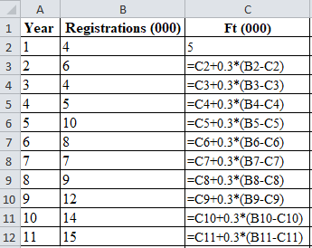
Calculation of forecast for year 2:
To calculate the forecast for year 2, substitute the value of the forecast of year 1, smoothing constant, and difference of actual and forecasted demand in the above formula. The result of forecast for year 2 is 4.70
Calculation of forecast for year 3:
To calculate the forecast for year 3, substitute the value of the forecast of year 1, smoothing constant, and difference of actual and forecasted demand in the above formula. The result of forecast for year 3 is 5.09
Calculation of forecast for year 4:
To calculate the forecast for year 4, substitute the value of the forecast of year 3, smoothing constant, and difference of actual and forecasted demand in the above formula. The result of forecast for year 3 is 4.763
Calculation of forecast for year 5:
To calculate the forecast for year 5, substitute the value of the forecast of year 4, smoothing constant, and difference of actual and forecasted demand in the above formula. The result of forecast for year 5 is 4.834
Calculation of forecast for year 6:
To calculate the forecast for year 6, substitute the value of the forecast of year 5, smoothing constant, and difference of actual and forecasted demand in the above formula. The result of forecast for year 5 is 6.384
Calculation of forecast for year 7:
To calculate the forecast for year 7, substitute the value of the forecast of year 6, smoothing constant, and difference of actual and forecasted demand in the above formula. The result of forecast for year 7 is 6.869
Calculation of forecast for year 8:
To calculate the forecast for year 8, substitute the value of the forecast of year 7, smoothing constant, and difference of actual and forecasted demand in the above formula. The result of forecast for year 8 is 6.908
Calculation of forecast for year 9:
To calculate the forecast for year 9, substitute the value of the forecast of year 8, smoothing constant, and difference of actual and forecasted demand in the above formula. The result of forecast for year 8 is 7.536
Calculation of forecast for year 10:
To calculate the forecast for year 10, substitute the value of the forecast of year 9, smoothing constant, and difference of actual and forecasted demand in the above formula. The result of forecast for year 9 is 8.875
Calculation of forecast for year 11:
To calculate the forecast for year 11, substitute the value of the forecast of year 10, smoothing constant, and difference of actual and forecasted demand in the above formula. The result of forecast for year 10 is 10.412
The forecasted value of registrations using exponential smoothing is provided in table 1
Calculation of MAD using exponential smoothing
Formula to calculate MAD
Table 1 provides the adequate forecasted data to compute MAD.
| Year | Registrations (000) | Ft (000) | Absolute error |
| 1 | 4 | 5.000 | 1 |
| 2 | 6 | 4.700 | 1.30 |
| 3 | 4 | 5.090 | 1.09 |
| 4 | 5 | 4.763 | 0.24 |
| 5 | 10 | 4.834 | 5.17 |
| 6 | 8 | 6.384 | 1.62 |
| 7 | 7 | 6.869 | 0.13 |
| 8 | 9 | 6.908 | 2.09 |
| 9 | 12 | 7.536 | 4.46 |
| 10 | 14 | 8.875 | 5.13 |
| 11 | 15 | 10.412 | 4.59 |
| Total | 26.81 | ||
| MAD | 2.44 |
Table 2
Excel calculation:
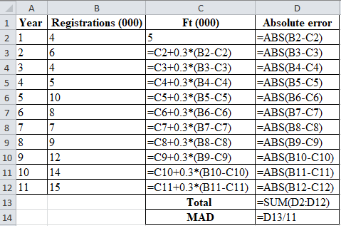
Mean Absolute Deviation:
Mean Absolute Deviation is obtained by dividing the summation of absolute values by the number of years. Absolute error is obtained by taking modulus for the difference between actual and forecasted values.
Calculation of absolute error for year 1
The absolute error for year 1 is the modulus of the difference between 4 and 5, which corresponds to 1. Therefore absolute error for year 1 is 1.
Calculation of absolute error for year 2
The absolute error for year 2 is the modulus of the difference between 6 and 4.7, which corresponds to 1.30. Therefore absolute error for year 2 is 1.30
Calculation of absolute error for year 3
The absolute error for year 3 is the modulus of the difference between 4 and 5.09, which corresponds to 1.09. Therefore absolute error for year 1.09
Calculation of absolute error for year 4
The absolute error for year 4 is the modulus of the difference between 5 and 4.763, which corresponds to 0.24. Therefore absolute error for year 4 is 0.24
Calculation of absolute error for year 5
The absolute error for year 5 is the modulus of the difference between 10 and 4.834, which corresponds to 5.17. Therefore absolute error for year 5 is 5.17
Calculation of absolute error for year 6
The absolute error for year 6 is the modulus of the difference between 8 and 6.384, which corresponds to 1.62. Therefore absolute error for year is 1.62
Calculation of absolute error for year 7
The absolute error for year 7 is the modulus of the difference between 7 and 6.869, which corresponds to 0.13. Therefore absolute error for year is 0.13
Calculation of absolute error for year 8
The absolute error for year 8 is the modulus of the difference between 9 and 6.908, which corresponds to 2.09. Therefore absolute error for year is 2.09
Calculation of absolute error for year 9
The absolute error for year 9 is the modulus of the difference between 12 and 7.536, which corresponds to 4.46. Therefore absolute error for year is 4.46
Calculation of absolute error for year 10
The absolute error for year 10 is the modulus of the difference between14 and 8.875, which corresponds to 5.13. Therefore absolute error for year is 5.13
Calculation of absolute error for year 11
The absolute error for year 11 is the modulus of the difference between 15 and 10.412, which corresponds to 4.59. Therefore absolute error for year is 4.59
Calculation of MAD using exponential smoothing
Upon substitution of summation, the value of absolute error for 11 years, that is, 26.81 is divided by number of years, that is, 11 yields MAD of 2.44
Hence, using exponential smoothing, the registrations at the seminar are forecasted and the computed MAD is 2.44
b)
To determine: Forecast the registrations at the seminar using exponential smoothing and hence compute MSE.
Answer to Problem 11P
Using exponential smoothing, the registrations at the seminar are forecasted and the computed MSE is 9.53
Explanation of Solution
Given information:
| Year | Registrations (000) |
| 1 | 4 |
| 2 | 6 |
| 3 | 4 |
| 4 | 5 |
| 5 | 10 |
| 6 | 8 |
| 7 | 7 |
| 8 | 9 |
| 9 | 12 |
| 10 | 14 |
| 11 | 15 |
Formula to calculate MSE
Table 1 provides the required forecasted data which in turn is used to compute MSE.
| Year | Registrations (000) | Ft (000) | Error2 |
| 1 | 4 | 5 | 1 |
| 2 | 6 | 4.700 | 1.69 |
| 3 | 4 | 5.090 | 1.19 |
| 4 | 5 | 4.763 | 0.06 |
| 5 | 10 | 4.834 | 26.69 |
| 6 | 8 | 6.384 | 2.61 |
| 7 | 7 | 6.869 | 0.02 |
| 8 | 9 | 6.908 | 4.38 |
| 9 | 12 | 7.536 | 19.93 |
| 10 | 14 | 8.875 | 26.27 |
| 11 | 15 | 10.412 | 21.05 |
| Total | 104.87 | ||
| MSE | 9.53 |
Table 3
Excel calculation:
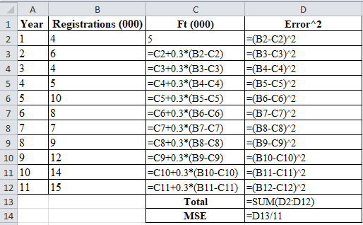
Error is the difference between actual and forecasted values. Table 2 provides the value of Error for the forecasted and given values.
Calculation of MSE
MSE is obtained by dividing the summation of the square of error (refer to Table (3)) with the n number of periods, that is, 11.
Hence, using exponential smoothing, the registrations at the seminar are forecasted and the computed MSE is 9.53.
Want to see more full solutions like this?
Chapter 4 Solutions
EBK PRINCIPLES OF OPERATIONS MANAGEMENT


- Can you guys help me with this? Thank you! Here's the question: Compared to the CONSTRAINT model, how has the network changed? How do you plan to add contingency to your network? Please answer this thoroughly Here's the what-if scenario: Assume that the LA warehouse becomes temporarily or even indefinitely disabled since facing a large-scale labor disruption. Re-optimize the network considering this new constraint. Here's the scenario comparison analysis: Scenario Constraint Scenario vs What-if Scenario Summary The Constraint Scenario exhibits a higher total cost of $7,424,575.45 compared to the What-if Scenario's total cost of $6,611,905.60, signifying a difference of approximately $812,669.85, which indicates a more expensive operation in the Constraint Scenario. The average service time is slightly higher in the Constraint Scenario (0.72 days vs. 0.70 days), suggesting that the What-if Scenario provides a marginally quicker service. Moreover, the average end-to-end service time…arrow_forwardCan you guys help me with this? Thank you! Here's the question: Compared to the CONSTRAINT model, how has the network changed? How do you plan to add contingency to your network? Please answer this throughly Here's the what-if scenario: Assume that Dallas plant has lost power. It cannot serve the DCs anymore and has to remain locked indefinitely. Re-optimize the network considering this new constraint. Here's the scenario comparison analysis: Scenario Constraint Scenario vs What-if Scenario Summary In comparing the Constraint Scenario to the What-if Scenario, a few key differences highlight the efficiencies evident in the supply chain. Firstly, the total cost in the Constraint Scenario is lower at $7,424,575.45, while the What-if Scenario incurs a total cost of $7,486,369.12, resulting in a cost delta of $61,793.67. Additionally, although both scenarios exhibit the same average service time of 0.72 days, the What-if Scenario has a more favorable average end-to-end service time of 2.41…arrow_forwardEmployee In-Service Training ASSIGNMENT: In-Service Training. The intern is required to plan and implement two in-service training sessions for employees. Each in-service should last at least 10 but not more than 30 minutes and should be given to all employees affected. The preceptor or supervisor/unit manager must approve all in-service topics. 1) One presentation should be related to a policy or procedure of any kind (e.g. proper use of equipment); 2) The second presentation must be related to sanitation or safety. For each in-service presentation, the intern must develop a written class plan and a visual aid (may be a handout, poster, PowerPoint slide presentation, etc.) appropriate to the life experiences, cultural diversity and educational background of the target audience. The intern must also measure behavior change. Note, this cannot be measured by a written pre- and post- test. That would be measuring knowledge. The intern mustactually observe and document that the learners…arrow_forward
- A small furniture manufacturer produces tables and chairs. Each product must go through three stages of the manufacturing process – assembly, finishing, and inspection. Each table requires 3 hours of assembly, 2 hours of finishing, and 1 hour of inspection. The profit per table is $120 while the profit per chair is $80. Currently, each week there are 200 hours of assembly time available, 180 hours of finishing time, and 40 hours of inspection time. Linear programming is to be used to develop a production schedule. Define the variables as follows: T = number of tables produced each week C= number of chairs produced each week According to the above information, what would the objective function be? (a) Maximize T+C (b) Maximize 120T + 80C (c) Maximize 200T+200C (d) Minimize 6T+5C (e) none of the above According to the information provided in Question 17, which of the following would be a necessary constraint in the problem? (a) T+C ≤ 40 (b) T+C ≤ 200 (c) T+C ≤ 180 (d) 120T+80C ≥ 1000…arrow_forwardAs much detail as possible. Dietary Management- Nursing Home Don't add any fill-in-the-blanksarrow_forwardMenu Planning Instructions Use the following questions and points as a guide to completing this assignment. The report should be typed. Give a copy to the facility preceptor. Submit a copy in your Foodservice System Management weekly submission. 1. Are there any federal regulations and state statutes or rules with which they must comply? Ask preceptor about regulations that could prescribe a certain amount of food that must be kept on hand for emergencies, etc. Is the facility accredited by any agency such as Joint Commission? 2. Describe the kind of menu the facility uses (may include standard select menu, menu specific to station, non-select, select, room service, etc.) 3. What type of foodservice does the facility have? This could be various stations to choose from, self-serve, 4. conventional, cook-chill, assembly-serve, etc. Are there things about the facility or system that place a constraint on the menu to be served? Consider how patients/guests are served (e.g. do they serve…arrow_forward
 MarketingMarketingISBN:9780357033791Author:Pride, William MPublisher:South Western Educational Publishing
 Contemporary MarketingMarketingISBN:9780357033777Author:Louis E. Boone, David L. KurtzPublisher:Cengage Learning
 Purchasing and Supply Chain ManagementOperations ManagementISBN:9781285869681Author:Robert M. Monczka, Robert B. Handfield, Larry C. Giunipero, James L. PattersonPublisher:Cengage Learning
 Practical Management ScienceOperations ManagementISBN:9781337406659Author:WINSTON, Wayne L.Publisher:Cengage,