
Concept explainers
Videos
At you can see in the following table, demand for heart transplant surgery at Washington General Hospital has increased steadily in the past few years:
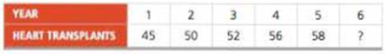
The director of medical services predicted 6 years ago that demand in year 1 would be 41 surgeries.
a) Use exponential smoothing, first with a smoothing constant of .6 and then with one of .9, to develop forecasts for years 2 through 6.
b) Use a 3-year moving average to forecast demand in years 4, 5, and 6.
c) Use the trend-projection method to forecast demand in years 1 through 6.
d) With MAD as the criterion, which of the four
a)
To determine: Findthe forecast for years 2 through 6, using exponential smoothing.
Introduction: A sequence of data pointing in successive order is known as time series. Time series forecasting is the prediction based on past events which are at a uniform time interval. Moving average method and trend projections are one of the time series methods which use weights to prioritize past data.
Answer to Problem 13P
The forecast for years 2 through 6 using exponential smoothing with smoothing constant 0.6 is 56.263 and smoothing constant 0.9 is 57.757.
Explanation of Solution
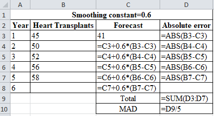
Forecast for years 1 through 6 using exponential smoothing with smoothing constant 0.6:
Given information:
| Year | 1 | 2 | 3 | 4 | 5 | 6 |
| Heart Transplants | 45 | 50 | 52 | 56 | 58 |
Formula to calculate the forecasted demand:
Where,
| Smoothing constant=0.6 | |||
| Year | Heart Transplants | Forecast | Absolute error |
| 1 | 45 | 41 | 4.000 |
| 2 | 50 | 43.400 | 6.600 |
| 3 | 52 | 47.360 | 4.640 |
| 4 | 56 | 50.144 | 5.856 |
| 5 | 58 | 53.658 | 4.342 |
| 6 | 56.263 | ||
| Total | 25.438 | ||
| MAD | 5.08768 | ||
Excel worksheet:
Calculation of the forecast for year 2:
To calculate forecast for year 2, substitute the value of forecast of year 1, smoothing constant and difference of actual and forecasted demand in the above formula. The result of the forecast for year 2 is 43.40.
Calculation of the forecast for year 3:
To calculate forecast for year 3, substitute the value of forecast of year 2, smoothing constant and difference of actual and forecasted demand in the above formula. The result of the forecast for year 3 is 47.360.
Calculation of the forecast for year 4:
To calculate forecast for year 4, substitute the value of forecast of year 3, smoothing constant and difference of actual and forecasted demand in the above formula. The result of the forecast for year 4 is 50.144.
Calculation of the forecast for year 5:
To calculate forecast for year 5, substitute the value of forecast of year 4, smoothing constant and difference of actual and forecasted demand in the above formula. The result of the forecast for year 5 is 53.658.
Calculation of the forecast for year 6:
To calculate forecast for year 6, substitute the value of forecast of year 5, smoothing constant and difference of actual and forecasted demand in the above formula. The result of the forecast for year 6 is 56.263.
Calculation of MAD using exponential smoothing with smoothing constant α=0.6:
Formula to calculate the Mean Absolute Deviation:
Calculation of the absolute error for year 1:
The absolute error for year 1 is the modulus of the difference between 45 and 41, which corresponds to 4. Therefore, the absolute error for year 1 is 4.
Calculation of the absolute error for year 2:
The absolute error for year 2 is the modulus of the difference between 50 and 43.4, which corresponds to 6.6. Therefore, the absolute error for year 2 is 6.6.
Calculation of the absolute error for year 3:
The absolute error for year 3 is the modulus of the difference between 52 and 47.360, which corresponds to 4.640. Therefore, the absolute error for year 3 is4.640.
Calculation of the absolute error for year 4:
The absolute error for year 4 is the modulus of the difference between 56 and 50.144, which corresponds to 5.856. Therefore, the absolute error for year 4 is5.856.
Calculation of the absolute error for year 5:
The absolute error for year 5 is the modulus of the difference between 58 and 53.658, which corresponds to 4.342. Therefore, the absolute error for year 5 is 4.342.
Calculation of the Mean Absolute Deviation using exponential smoothing:
Upon the substitution of summation value of absolute error for 5 years, that is, 25.438 are divided by number of years. That is, 5 yields MAD of 5.08768.
The forecast for years 2 through 6 using exponential smoothing with 0.6 as smoothing constant is 56.263.
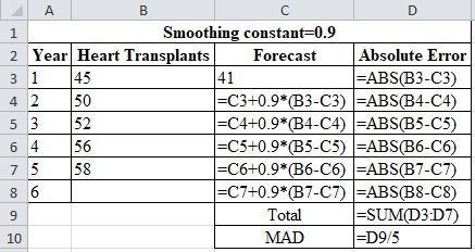
The forecast for years 1 through 6 using exponential smoothing with smoothing constant 0.9:
Given information:
| Year | 1 | 2 | 3 | 4 | 5 | 6 |
| Heart Transplants | 45 | 50 | 52 | 56 | 58 |
Formula to calculate the forecasted demand:
Where
| Smoothing constant=0.9 | |||
| Year | Heart Transplants | Forecast | Absolute Error |
| 1 | 45 | 41 | 4 |
| 2 | 50 | 44.600 | 5.400 |
| 3 | 52 | 49.460 | 2.540 |
| 4 | 56 | 51.746 | 4.254 |
| 5 | 58 | 55.575 | 2.425 |
| 6 | 57.757 | 57.757 | |
| Total | 18.6194 | ||
| MAD | 3.72388 | ||
Excel worksheet:
Calculation of the forecast for year 2:
To calculate the forecast for year 2, substitute the value of forecast of year 1, smoothing constant and difference of actual and forecasted demand in the above formula. The result of the forecast for year 2 is 44.60.
Calculation of the forecast for year 3:
To calculate forecast for year 3, substitute the value of forecast of year 2, smoothing constant and difference of actual and forecasted demand in the above formula. The result of the forecast for year 3 is 49.460.
Calculation of the forecast for year 4:
To calculate forecast for year 4, substitute the value of forecast of year 3, smoothing constant and difference of actual and forecasted demand in the above formula. The result of the forecast for year 4 is 50.144.
Calculation of the forecast for year 5:
To calculate forecast for year 5, substitute the value of forecast of year 4, smoothing constant and difference of actual and forecasted demand in the above formula. The result of the forecast for year 5 is55.575.
Calculation of the forecast for year 6:
To calculate forecast for year 6, substitute the value of forecast of year 5, smoothing constant and difference of actual and forecasted demand in the above formula. The result of the forecast for year 6 is57.757.
Calculation of MAD using exponential smoothing with smoothing constant α=0.9:
Formula to calculate the Mean Absolute Deviation:
Calculation of the absolute error for year 1:
The absolute error for year 1 is the modulus of the difference between 45 and 41, which corresponds to 4. Therefore, the absolute error for year 1 is 4.
Calculation of the absolute error for year 2:
The absolute error for year 2 is the modulus of the difference between 50 and 44.6, which corresponds to 5.4. Therefore, the absolute error for year 2 is 5.4.
Calculation of the absolute error for year 3:
The absolute error for year 3 is the modulus of the difference between 52 and49.460, which corresponds to 2.540. Therefore, the absolute error for year 3 is2.540.
Calculation of the absolute error for year 4:
The absolute error for year 4 is the modulus of the difference between 56 and51.746, which corresponds to 4.254. Therefore, the absolute error for year 4 is4.254.
Calculation of the absolute error for year 5:
The absolute error for year 5 is the modulus of the difference between 58 and55.575, which corresponds to 2.425. Therefore, the absolute error for year 5 is 2.425.
Calculation of the Mean Absolute Deviation using exponential smoothing:
Upon the substitution of summation value of absolute error for 5 years, that is,18.6194are divided by the number of years. That is, 5 yields MAD of 3.72388.
The forecast for years 2 through 6 using exponential smoothing with 0.9 as smoothing constant is 57.757.
Hence, the forecast for years 2 through 6 using exponential smoothing with smoothing constant 0.6 is 56.263 and smoothing constant 0.9 is 57.757.
b)
To determine: Using 3-year moving average, forecast the demand for years 4, 5 and 6.
Answer to Problem 13P
The demand forecast for years 4, 5 and 6 is 49, 52.67 and 55.33.
Explanation of Solution
Given information:
| Year | 1 | 2 | 3 | 4 | 5 | 6 |
| Heart Transplants | 45 | 50 | 52 | 56 | 58 |
Formula to calculate the forecasted demand:
| Year | Heart Transplants | Forecast | Absolute Error |
| 1 | 45 | ||
| 2 | 50 | ||
| 3 | 52 | ||
| 4 | 56 | 49 | 7 |
| 5 | 58 | 52.67 | 5.333 |
| 6 | 55.33 | ||
| Total | 12.333 | ||
| MAD | 6.1667 |
Excel worksheet:
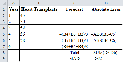
Calculation of the forecast for year 4:
To calculate the forecast for year 4, divide the summation of the values from years 1, 2 and 3 and divide by 3. The corresponding value 49 is the forecast for year 4. The 3-year moving average for year 4 is 49.
Calculation of the forecast for year 5:
To calculate the forecast for year 5, divide the summation of the values from years 2, 3 and 4 and divide by 3. The corresponding value 52.67 is the forecast for year 5. The 3-year moving average for year 5 is 52.67.
Calculation of the forecast for year 6:
To calculate the forecast for year 6, divide the summation of the values from years 3, 4, 5 and divide by 3. The corresponding value 55.33 is the forecast for year 5. The 3-year moving average for year 5 is 55.33.
Calculation of MAD using 3-year moving average:
Formula to calculate the Mean Absolute Deviation:
Calculation of the absolute error for year 4:
The absolute error for year 4 is the modulus of the difference between 56 and 49, which corresponds to 7. Therefore, the absolute error for year 4 is 7.
Calculation of the absolute error for year 5:
The absolute error for year 4 is the modulus of the difference between 58 and 52.67, which corresponds to 5.33. Therefore, the absolute error for year 4 is 5.33.
Calculation of the Mean Absolute Deviation using 3-year moving average:
Upon the substitution of the summation value of the absolute error for 2 years, that is,12.333is divided by number of years. That is, 2 yields MAD of 6.1666.
Hence, the demand forecast for years 4, 5 and 6 is 49, 52.67 and 55.33.
c)
To determine: Find the demand forecast in year 1 through 6using trend projection.
Answer to Problem 13P
The forecast in year 1 through 6using trend projection is62.1.
Explanation of Solution
Given information:
| Year | 1 | 2 | 3 | 4 | 5 | 6 |
| Heart Transplants | 45 | 50 | 52 | 56 | 58 |
Formula to calculate the demand forecast
Where,
Where,
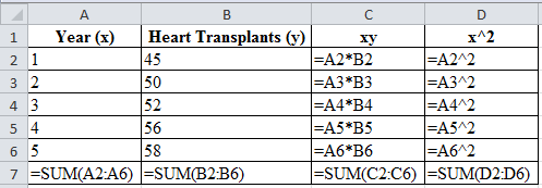
| Year (x) | Heart Transplants (y) | xy | x^2 |
| 1 | 45 | 45 | 1 |
| 2 | 50 | 100 | 4 |
| 3 | 52 | 156 | 9 |
| 4 | 56 | 224 | 16 |
| 5 | 58 | 290 | 25 |
| ∑=15 | ∑=261 | ∑=815 | ∑=55 |
Excel worksheet
Substituting the values in the above formula
Calculation of average of x values
The average of x values is obtained by dividing the summation of x values, that is, (1+2+…+5) with the number of period n. That is, 5. The value of
Calculation of average of y values
The average of y values is obtained by dividing the summation of sales with the number of period n. That is, 5. The value of
Calculation of slope of regression line‘b’:
The summation of product of sales (y) with x values is ∑xy = 815, the product of number of years (n), the average of x values and the average of y values is obtained. That is,
The summation of square of x values, that is, 55 is subtracted from the product of the number of years. That is,5 with average of x values;3. The resultant value is 10. The slope of regression line is obtained by dividing 32 with 10. The value of ‘b’ is 3.2.
Calculation of y-axis intercept ‘a’:
The y-axis intercept is obtained by the difference between average of y values and values obtained by the product of slope of regression line with average of x values. The resultant value of ‘a’ is 42.9.
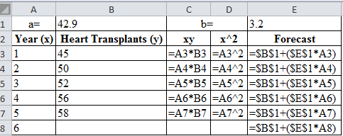
Calculation of the forecast for years 1 through 6:
| a= | 42.9 | b= | 3.2 | |
| Year (x) | Heart Transplants (y) | xy | x^2 | Forecast |
| 1 | 45 | 45 | 1 | 46.1 |
| 2 | 50 | 100 | 4 | 49.3 |
| 3 | 52 | 156 | 9 | 52.5 |
| 4 | 56 | 224 | 16 | 55.7 |
| 5 | 58 | 290 | 25 | 58.9 |
| 6 | 62.1 | |||
Excel worksheet:
Calculation of forecast of year 1:
The forecast for year 1 is obtained by the summation of the product of slope of regression line and forecasted year, with the y-axis intercept. The forecasted value obtained is 46.1.
Calculation of forecast of year 2:
The forecast for year 2 is obtained by the summation of the product of slope of regression line and forecasted year, with the y-axis intercept. The forecasted value obtained is 49.3.
Calculation of forecast of year 3:
The forecast for year 3 is obtained by the summation of the product of slope of regression line and forecasted year, with the y-axis intercept. The forecasted value obtained is 52.5.
Calculation of forecast of year 4:
The forecast for year 4 is obtained by the summation of the product of slope of regression line and forecasted year, with the y-axis intercept. The forecasted value obtained is 55.7.
Calculation of forecast of year 5:
The forecast for year 5 is obtained by the summation of the product of slope of regression line and forecasted year, with the y-axis intercept. The forecasted value obtained is 58.9.
Calculation of forecast of year 6:
The forecast for year 6 is obtained by the summation of the product of slope of regression line and forecasted year, with the y-axis intercept. The forecasted value obtained is 62.1.
Formula to calculate the Mean Absolute Deviation:
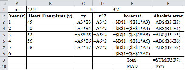
Calculation of MAD using trend projection:
| a= | 42.9 | b= | 3.2 | ||
| Year (x) | Heart Transplants (y) | xy | x^2 | Forecast | Absolute error |
| 1 | 45 | 45 | 1 | 46.1 | 1.1 |
| 2 | 50 | 100 | 4 | 49.3 | 0.7 |
| 3 | 52 | 156 | 9 | 52.5 | 0.5 |
| 4 | 56 | 224 | 16 | 55.7 | 0.3 |
| 5 | 58 | 290 | 25 | 58.9 | 0.9 |
| 6 | 62.1 | ||||
| Total | 3.5 | ||||
| MAD | 0.7 | ||||
Excel worksheet:
Calculation of the absolute error for year 1:
The absolute error for year 1 is the modulus of the difference between 45 and 46.1, which corresponds to 1.1. Therefore, the absolute error for year 1 is 1.1.
Calculation of the absolute error for year 2:
The absolute error for year 2 is the modulus of the difference between 50 and 49.3, which corresponds to 0.7. Therefore, the absolute error for year 2 is 0.7.
Calculation of the absolute error for year 3:
The absolute error for year 3 is the modulus of the difference between 52 and 52.5, which corresponds to 0.5. Therefore, the absolute error for year 3 is 0.5.
Calculation of the absolute error for year 4:
The absolute error for year 4 is the modulus of the difference between 56 and 55.7, which corresponds to 0.3. Therefore, the absolute error for year 4 is 0.3.
Calculation of the absolute error for year 5:
The absolute error for year 5 is the modulus of the difference between 58 and 58.9, which corresponds to 0.9. Therefore, the absolute error for year 5 is 0.9.
Calculation of the Mean Absolute Deviation using trend projection:
Upon the substitution of summation value of absolute error for 5 years, that is,3.5is divided by the number of years. That is,5 yields MAD of 0.7.
Thus, the forecast in year 1 through 6 using trend projection is 62.1.
d)
To determine: Compare the MAD of exponential smoothing, 3-year moving average and trend projection and infer the best method.
Explanation of Solution
On Comparing MAD from the four methods, (refer to equations (1), (2), (3) and (4)) it can be inferred that trend projection is the best methods since it has the least MAD.
Want to see more full solutions like this?
Chapter 4 Solutions
EBK PRINCIPLES OF OPERATIONS MANAGEMENT


- Do you feel there is anything positive about rework?arrow_forwardDo you think technology can achieve faster setup times? How would it be implemented in the hospital workforce?arrow_forwardIn your experience or opinion, do you think process changes like organizing workspaces make a bigger difference, or is investing in technology usually the better solution for faster setups?arrow_forward
- Have you seen rework done in your business, and what was done to prevent that from occurring again?arrow_forwardResearch a company different than case studies examined and search the internet and find an example of a business that had to rework a process. How was the organization affected to rework a process in order to restore a good flow unit? Did rework hurt a process or improve the organization's operational efficiency? • Note: Include a reference with supportive citations in the discussion reply in your post.arrow_forwardSetup time is very important in affecting a process and the capacity of a process. How do you reduce setup time? Give examples of reducing setup time. Please Provide a referenecearrow_forward
- Do you think TPS was successful? If so, how? Are there other companies that have used TPS? If so, give examples. Please provide a referencearrow_forwardGiven the significant impact on finances, production timelines, and even equipment functionality, as you pointed out, what do you believe is the most effective single strategy a company can implement to significantly reduce the occurrence of rework within their operations?arrow_forwardDurban woman, Nombulelo Mkumla, took to social media last week to share how she discovered the rodent.In a lengthy Facebook post, she said she purchased the loaf of bread from a local shop after work on August 27.For the next days, Mkumla proceeded to use slices of bread from the load to make toast."Then, on the morning of August 31, I took the bread out of the fridge to make toast and noticed something disgusting andscary. I took a picture and sent it to my friends, and one of them said, 'Yi mpuku leyo tshomi' [That's a rat friend]“."I was in denial and suggested it might be something else, but the rat scenario made sense - it's possible the rat got into thebread at the factory, and no one noticed," Mkumla said.She went back to the shop she'd bought the bread from and was told to lay a complaint directly with the supplier.She sent an email with a video and photographs of the bread.Mkumla said she was later contacted by a man from Sasko who apologised for the incident.According to…arrow_forward
- PepsiCo South Africa says the incident where a woman discovered part of a rodent in her loaf of bread, is anisolated occurrence.Durban woman, Nombulelo Mkumla, took to social media last week to share how she discovered the rodent.In a lengthy Facebook post, she said she purchased the loaf of bread from a local shop after work on August 27.For the next days, Mkumla proceeded to use slices of bread from the load to make toast."Then, on the morning of August 31, I took the bread out of the fridge to make toast and noticed something disgusting andscary. I took a picture and sent it to my friends, and one of them said, 'Yi mpuku leyo tshomi' [That's a rat friend]“."I was in denial and suggested it might be something else, but the rat scenario made sense - it's possible the rat got into thebread at the factory, and no one noticed," Mkumla said.She went back to the shop she'd bought the bread from and was told to lay a complaint directly with the supplier.She sent an email with a video and…arrow_forwardDurban woman, Nombulelo Mkumla, took to social media last week to share how she discovered the rodent.In a lengthy Facebook post, she said she purchased the loaf of bread from a local shop after work on August 27.For the next days, Mkumla proceeded to use slices of bread from the load to make toast."Then, on the morning of August 31, I took the bread out of the fridge to make toast and noticed something disgusting andscary. I took a picture and sent it to my friends, and one of them said, 'Yi mpuku leyo tshomi' [That's a rat friend]“."I was in denial and suggested it might be something else, but the rat scenario made sense - it's possible the rat got into thebread at the factory, and no one noticed," Mkumla said.She went back to the shop she'd bought the bread from and was told to lay a complaint directly with the supplier.She sent an email with a video and photographs of the bread.Mkumla said she was later contacted by a man from Sasko who apologised for the incident.According to…arrow_forwardRead the project statement and answer ALL of the questions that follow PROJECT STATEMENT The African Integrated High-Speed Railway Network (AIHSRN). African nations are preparing to invest billions in a significant overhaul of their rail infrastructure as part of an ambitious plan for the continent. One of the key projects underway is the African Integrated High-Speed Railway Network (AIHSRN), which aims to connect Africa's capital cities and major commercial centres with a high-speed railway network to enhance continental trade and competition. This network will span 2,000 km (1,243 miles) and connect 60 cities, including Nairobi, Lagos, Cairo, and Dakar. It will improve access to essential markets, enhance economic cooperation, and encourage regional collaboration. The plan is poised to revolutionise intra-African trade by reducing travel times and lowering transportation costs, making trade between African nations more competitive. The trains will be capable of reaching speeds of up…arrow_forward
 Contemporary MarketingMarketingISBN:9780357033777Author:Louis E. Boone, David L. KurtzPublisher:Cengage Learning
 MarketingMarketingISBN:9780357033791Author:Pride, William MPublisher:South Western Educational Publishing
 Practical Management ScienceOperations ManagementISBN:9781337406659Author:WINSTON, Wayne L.Publisher:Cengage,
 Purchasing and Supply Chain ManagementOperations ManagementISBN:9781285869681Author:Robert M. Monczka, Robert B. Handfield, Larry C. Giunipero, James L. PattersonPublisher:Cengage Learning