Videos
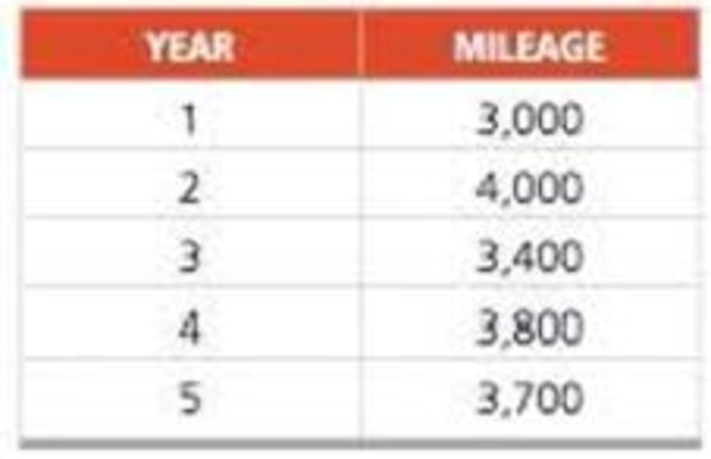
The Carbondale Hospital is considering the purchase of a new ambulance. The decision will rest partly on the anticipated mileage to be driven next year. The miles driven during the past 5 years are as follows:
a) Forecast the mileage for next year (6th year) using a 2-year moving average.
b) Find the MAD based on the 2-year moving average. (Hint: You will have only 3 years of matched data.)
c) Use a weighted 2-year moving average with weights of .4 and .6 to forecast next year’s mileage. (The weight of .6 is for the most recent year.) What MAD results from using this approach to
d) Compute the forecast for year 6 using exponential smoothing, an initial forecast for year 1 of 3,000 miles, and α = .5.
a)
To determine: Using 2-year moving average, forecast the mileage for the 6th year.
Introduction: Forecasting is used to predict future changes or demand patterns. It involves different approaches and varies with different time periods. A sequence of data points in successive order is known as a time series. Time series forecasting is the prediction based on past events which are at a uniform time interval.
Answer to Problem 5P
The forecasted mileage for the 6th year is 3,750.
Explanation of Solution
Given information:
| Year | Mileage |
| 1 | 3,000 |
| 2 | 4,000 |
| 3 | 3,400 |
| 4 | 3,800 |
| 5 | 3,700 |
Formula to forecast the mileage for the 6th year:
| Year | Mileage | Moving Average |
| 1 | 3,000 | |
| 2 | 4,000 | |
| 3 | 3,400 | 3,500 |
| 4 | 3,800 | 3,700 |
| 5 | 3,700 | 3,600 |
| 6 | 3,750 |
Excel worksheet:
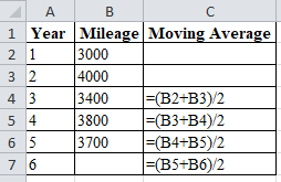
Calculation of the mileage forecast for the 6th year:
The mileage forecast for the 6th year is obtained by summing up the mileage for the 4th and 5thyears and dividing the sum by the
The forecast for the 6th year is 3,750.
Hence, using 2-year moving average, the mileage forecast for the 6th year is 3,750
b)
To determine: The computation of the Mean Average Deviation (MAD) using 2-year moving average.
Answer to Problem 5P
Mean Average Deviation (MAD) using 2-year moving average is 100
Explanation of Solution
Given information:
| Year | Mileage |
| 1 | 3,000 |
| 2 | 4,000 |
| 3 | 3,400 |
| 4 | 3,800 |
| 5 | 3,700 |
Formula to compute MAD:
| Year | Mileage | Moving Average | Error | Absolute Error |
| 1 | 3,000 | |||
| 2 | 4,000 | |||
| 3 | 3,400 | 3,500 | -100 | 100 |
| 4 | 3,800 | 3,700 | 100 | 100 |
| 5 | 3,700 | 3,600 | 100 | 100 |
| Total | 300 | |||
| MAD | 100 |
Excel worksheet:
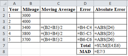
Calculation of the absolute error for year 3:
Moving average:
Error:
Absolute error:
To calculate the forecast for year 3, divide the summation of the values of year 1&2 by period n i.e. 2. The corresponding value is 3500 which is the forecast for the year 3.
Absolute Error for year 3 is the modulus of the difference between 3400 and 3500, which corresponds to 100. Therefore absolute error for year 3 is 100.
Calculation of the absolute error for year 4:
Moving average:
Error:
Absolute error:
To calculate the forecast for year 4, divide the summation of the values of year 2&3 by period n i.e. 2. The corresponding value is 3700 which is the forecast for the year 4.
Absolute Error for year 4 is the modulus of the difference between 3800 & 3700 which corresponds to 100. Therefore Absolute error for Year 4 is 100.
Calculation of the absolute error for year 5:
Moving average:
Error:
Absolute error:
To calculate the forecast for year 5, divide the summation of the values of year 3&4 by period n i.e. 2. The corresponding value is 3600 which is the forecast for the year 5.
Absolute Error for year 5 is the modulus of the difference between 3,700 & 3,600 which corresponds to 100. Therefore Absolute error for Year 5 is 100.
Calculation of the Mean Absolute Deviation:
Mean Absolute Deviation is obtained by dividing the summation of absolute values by the number of years. Absolute error is obtained by taking modulus for the difference between Actual and forecasted values.
Upon substitution of summation value of absolute error for 3 years i.e. 300 is divided by number of years i.e. 3 yields MAD of 100.
Hence, the computed Mean Average Deviation (MAD) using 2-year moving average is 100
c)
To determine: The mileage forecast for year 6 and also compute Mean Absolute Deviation (MAD) using weighted 2-year moving average with weights 0.4 and 0.6
Answer to Problem 5P
The forecast for year 6 and the Mean Absolute Deviation (MAD) using weighted moving averages are 3,741 & 139.67 respectively.
Explanation of Solution
Given information:
| Year | Mileage |
| 1 | 3,000 |
| 2 | 4,000 |
| 3 | 3,400 |
| 4 | 3,800 |
| 5 | 3,700 |
Formula to compute MAD:
| Year | Mileage | Weighted Moving Average | Error | Absolute Error |
| 1 | 3,000 | |||
| 2 | 4,000 | |||
| 3 | 3,400 | 3,601 | -201 | 201 |
| 4 | 3,800 | 3,641 | 159 | 159 |
| 5 | 3,700 | 3,641 | 59 | 59 |
| 6 | 3,741 | |||
| Total | 419 | |||
| MAD | 139.67 |
Excel worksheet:
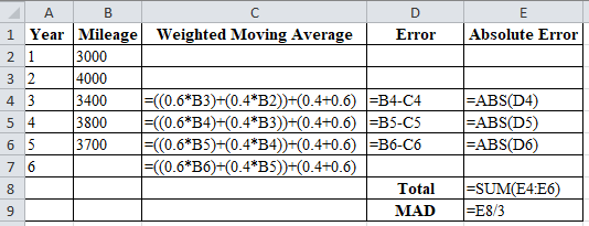
Calculation of the weighted moving average for year 3:
To calculate the forecast for year 3, multiply the weights with the mileage of recent year, i.e. multiply weight 0.6 with 4,000 and 0.4 with 3,000. Divide the summation of the multiplied values with the summation of the weights i.e. (0.6+0.4).
The corresponding result is 3,601 obtained is the forecasted value for year 3. Therefore, forecasted Weighted Moving Average for year 3 is 3,601.
Calculation of the weighted moving average for year 4:
To calculate the forecast for year 4, multiply the weights with the mileage of recent year, i.e. multiply weight 0.6 with 3,400 and 0.4 with 4,000. Divide the summation of the multiplied values with the summation of the weights i.e. (0.6+0.4).
The corresponding result is 3641 obtained is the forecasted value for year 4. Therefore, forecasted Weighted Moving Average for year 3 is 3,641.
Calculation of the weighted moving average for year 5:
To calculate the forecast for year 5, multiply the weights with the mileage of recent year, i.e. multiply weight 0.6 with 3,800 and 0.4 with 3,400. Divide the summation of the multiplied values with the summation of the weights i.e. (0.6+0.4).
The corresponding result is 3641 obtained is the forecasted value for year 5. Therefore, forecasted Weighted Moving Average for year 3 is 3,641.
Calculation of the weighted moving average for year 6:
To calculate the forecast for year 6, multiply the weights with the mileage of recent year, i.e. multiply weight 0.6 with 3,700 and 0.4 with 3,800. Divide the summation of the multiplied values with the summation of the weights i.e.
The corresponding result is 3,741 obtained is the forecasted value for year 6. Therefore, forecasted Weighted Moving Average for year 6 is 3,741.
Absolute Error:
Absolute error is the modulus of the difference between the values of actual and forecasted demand.
Calculation of the absolute error for year 3:
Absolute Error for year 3 is the modulus of the difference between 3400 and 3601, which corresponds to 201. Therefore absolute error for year 3is 201;
Calculation of the absolute error for year 4:
Absolute Error for year 4 is the modulus of the difference between 3800 and 3641, which corresponds to 159. The absolute error for year 4 is 159.
Calculation of the absolute error for year 5:
Absolute Error for year 5 is the modulus of the difference between 3,700 and 3,641, which corresponds to 59. The absolute error for year 5 is 59.
Calculation of the Mean Absolute Deviation:
Upon substitution of summation value of absolute error for 13 years i.e. 419 is divided by number of years i.e. 3 yields MAD of 139.67. Therefore, Mean Absolute Deviation =139.67
Hence, using weighted 2-year moving average with weights 0.4 and 0.6, the mileage forecast for year 6 and the computed Mean Absolute Deviation (MAD)are 3,741and 139.67,respectively.
d)
To determine: Using exponential smoothing technique, forecast the mileage for year 6.
Answer to Problem 5P
The mileage forecast for year 6 is 3,662.5
Explanation of Solution
Given information:
| Year | Mileage |
| 1 | 3,000 |
| 2 | 4,000 |
| 3 | 3,400 |
| 4 | 3,800 |
| 5 | 3,700 |
Formula to calculate the demand forecast:
Where,
| Year | Mileage | Forecast |
| 1 | 3,000 | 3,000 |
| 2 | 4,000 | 3,000 |
| 3 | 3,400 | 3,500 |
| 4 | 3,800 | 3,450 |
| 5 | 3,700 | 3,625 |
| 6 | 3,662.5 |
Excel worksheet:
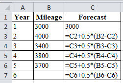
Calculation of the forecast for year 2:
To calculate forecast for the year 2, substitute the value of forecast of year 1, smoothing constant and difference of actual and forecasted mileage in the above formula. The result of forecast for year 2 is 3,000.
Calculation of the forecast for year 3:
To calculate forecast for the year 3, substitute the value of forecast of year 2, smoothing constant and difference of actual and forecasted mileage in the above formula. The result of forecast for year 3 is 3500.
Calculation of the forecast for year 4:
To calculate forecast for the year 4, substitute the value of forecast of year 3, smoothing constant and difference of actual and forecasted mileage in the above formula. The result of forecast for year 2 is 3,450.
Calculation of the forecast for year 5:
To calculate forecast for the year 5, substitute the value of forecast of year 4, smoothing constant and difference of actual and forecasted mileage in the above formula. The result of forecast for year 5 is 3,625.
Calculation of the forecast for year 6:
To calculate forecast for the year 6, substitute the value of forecast of year 5, smoothing constant and difference of actual and forecasted mileage in the above formula. The result of forecast for year 6 is 3,662.5.
Hence, using exponential smoothing technique, the forecast for year 6 is 3,662.5.
Want to see more full solutions like this?
Chapter 4 Solutions
EBK PRINCIPLES OF OPERATIONS MANAGEMENT


- Prepare a graph of the monthly forecasts and average forecast demand for Chicago Paint Corp., a manufacturer of specialized paint for artists. Compute the demand per day for each month (round your responses to one decimal place). Month B Production Days Demand Forecast Demand per Day January 21 950 February 19 1,150 March 21 1,150 April 20 1,250 May 23 1,200 June 22 1,000' July 20 1,350 August 21 1,250 September 21 1,050 October 21 1,050 November 21 December 225 950 19 850arrow_forwardThe president of Hill Enterprises, Terri Hill, projects the firm's aggregate demand requirements over the next 8 months as follows: 2,300 January 1,500 May February 1,700 June 2,100 March April 1,700 1,700 July August 1,900 1,500 Her operations manager is considering a new plan, which begins in January with 200 units of inventory on hand. Stockout cost of lost sales is $125 per unit. Inventory holding cost is $25 per unit per month. Ignore any idle-time costs. The plan is called plan C. Plan C: Keep a stable workforce by maintaining a constant production rate equal to the average gross requirements excluding initial inventory and allow varying inventory levels. Conduct your analysis for January through August. The average monthly demand requirement = units. (Enter your response as a whole number.) In order to arrive at the costs, first compute the ending inventory and stockout units for each month by filling in the table below (enter your responses as whole numbers). Ending E Period…arrow_forwardMention four early warning indicators that a business may be at risk.arrow_forward
- 1. Define risk management and explain its importance in a small business. 2. Describe three types of risks commonly faced by entrepreneurs. 3. Explain the purpose of a risk register. 4. List and briefly describe four risk response strategies. (5 marks) (6 marks) (4 marks) (8 marks) 5. Explain how social media can pose a risk to small businesses. (5 marks) 6. Identify and describe any four hazard-based risks. (8 marks) 7. Mention four early warning indicators that a business may be at risk. (4 marks)arrow_forwardState whether each of the following statements is TRUE or FALSE. 1. Risk management involves identifying, analysing, and mitigating risks. 2. Hazard risks include interest rate fluctuations. 3. Entrepreneurs should avoid all forms of risks. 4. SWOT analysis is a tool for risk identification. 5. Scenario building helps visualise risk responses. 6. Risk appetite defines how much risk an organisation is willing to accept. 7. Diversification is a risk reduction strategy. 8. A risk management framework must align with business goals. 9. Political risk is only relevant in unstable countries. 10. All risks can be eliminated through insurance.arrow_forward9. A hazard-based risk includes A. Political instability B. Ergonomic issues C. Market demand D. Taxation changesarrow_forward
 MarketingMarketingISBN:9780357033791Author:Pride, William MPublisher:South Western Educational Publishing
 Practical Management ScienceOperations ManagementISBN:9781337406659Author:WINSTON, Wayne L.Publisher:Cengage,
 Contemporary MarketingMarketingISBN:9780357033777Author:Louis E. Boone, David L. KurtzPublisher:Cengage Learning
 Purchasing and Supply Chain ManagementOperations ManagementISBN:9781285869681Author:Robert M. Monczka, Robert B. Handfield, Larry C. Giunipero, James L. PattersonPublisher:Cengage Learning