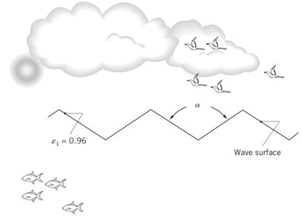
In Problems 12.20 and 12.25, we estimated the earth’s surface temperature, assuming the earth is black. Most of the earth’s surface is water, which has a hemispherical emissivity of ε = 0.96 . In reality, the water surface is not flat but has waves and ripples. (a) Assuming the wave geometry can be closely approximated as two-dimensional and as shown in the schematic, determine the effective emissivity of the water surface, as defined in Problem 13.43. for α = 3 π / 4 . (b) Calculate and plot the effective emissivity of the water surface, normalized by the hemispherical emissivity of water ( ε eff / ε ) over the range π / 2 ≤ α ≤ π .
In Problems 12.20 and 12.25, we estimated the earth’s surface temperature, assuming the earth is black. Most of the earth’s surface is water, which has a hemispherical emissivity of ε = 0.96 . In reality, the water surface is not flat but has waves and ripples. (a) Assuming the wave geometry can be closely approximated as two-dimensional and as shown in the schematic, determine the effective emissivity of the water surface, as defined in Problem 13.43. for α = 3 π / 4 . (b) Calculate and plot the effective emissivity of the water surface, normalized by the hemispherical emissivity of water ( ε eff / ε ) over the range π / 2 ≤ α ≤ π .
Solution Summary: The author calculates the effective emissivity of the water surface over the range of from 0 to 0.963. The Stefan's constant is 5.67108 W/m2
In Problems 12.20 and 12.25, we estimated the earth’s surface temperature, assuming the earth is black. Most of the earth’s surface is water, which has a hemispherical emissivity of
ε
=
0.96
. In reality, the water surface is not flat but has waves and ripples. (a) Assuming the wave geometry can be closely approximated as two-dimensional and as shown in the schematic, determine the effective emissivity of the water surface, as defined in Problem 13.43. for
α
=
3
π
/
4
. (b) Calculate and plot the effective emissivity of the water surface, normalized by the hemispherical emissivity of water
(
ε
eff
/
ε
)
over the range
π
/
2
≤
α
≤
π
.
Find the Laplace Transform of the following functions
1) f() cos(ar)
Ans. F(s)=7
2ws
2) f() sin(at)
Ans. F(s)=
s² + a²
3) f(r)-rcosh(at)
Ans. F(s)=
2as
4)(t)=sin(at)
Ans. F(s)=
2
5) f(1) = 2te'
Ans. F(s)=
(S-1)
5+2
6) (1) e cos()
Ans. F(s) =
(+2)+1
7) (1) (Acostẞr)+ Bsin(Br)) Ans. F(s)-
A(s+a)+BB
(s+a)+B
8) f()-(-)()
Ans. F(s)=
9)(1)(1)
Ans. F(s):
10) f(r),()sin()
Ans. F(s):
11)
2
k
12)
0
13)
0
70
ㄷ..
a 2a 3a 4a
2 3 4
14) f(1)=1,
0<1<2
15) (1) Ksin(t) 0
For Problems 5–19 through 5–28, design a crank-rocker mechanism with a time ratio of Q, throw angle of (Δθ4)max, and time per cycle of t. Use either the graphical or analytical method. Specify the link lengths L1, L2, L3, L4, and the crank speed.
Q = 1; (Δθ4)max = 78°; t = 1.2s.
3) find the required fillet welds size if the allowable
shear stress is 9.4 kN/m² for the figure below.
Calls
Ans: h=5.64 mm
T
=
حاجة
، منطقة
نصف القوة
250
190mm
450 mm
F= 30 KN
そのに青
-F₂= 10 KN
F2
Java: An Introduction to Problem Solving and Programming (8th Edition)
Knowledge Booster
Learn more about
Need a deep-dive on the concept behind this application? Look no further. Learn more about this topic, mechanical-engineering and related others by exploring similar questions and additional content below.


 Principles of Heat Transfer (Activate Learning wi...Mechanical EngineeringISBN:9781305387102Author:Kreith, Frank; Manglik, Raj M.Publisher:Cengage Learning