Concept explainers
Monitor the adjusted exponential smoothing
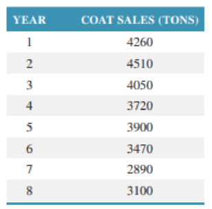
The Willow River Mining Company mines and ships coal. It has experienced the following demand for coal during the past eight years:

Develop an adjusted exponential smoothing model (α = .30, β = .20) and a linear trend line model, and compare the forecast accuracy of the two using MAD. Indicate which forecast seems to be most accurate.
Want to see the full answer?
Check out a sample textbook solution
Chapter 12 Solutions
Operations and Supply Chain Management 9th edition
Additional Business Textbook Solutions
Horngren's Cost Accounting: A Managerial Emphasis (16th Edition)
Financial Accounting, Student Value Edition (5th Edition)
PRIN.OF CORPORATE FINANCE
Corporate Finance (4th Edition) (Pearson Series in Finance) - Standalone book
MARKETING:REAL PEOPLE,REAL CHOICES
- I need to forecast using a 3-Period-Moving-Average-Monthly forecasting model which I did but then I need to use my forecast numbers to generate a Master Production Schedule (MPS) I have to Start with actual sales (my own test data numbers) for August-2022 Oct-2022 i need to create MPS to supply demand starting November-2022 April 2023 I just added numbers without applying formulas to the mps on the right side of the spreadsheet because I do not know how to do it. The second image is the example of what it should look like. Thank You.arrow_forwardSolve the following Question 1. How do volume and variety affect the process selection and layout types? Discuss 2. How is the human resource aspect important to operation function? Discuss 3. Discuss the supply network design and its impact on the overall performance of the organization.arrow_forwardHelp with question?arrow_forward
- What are some good examples of bullet points on a resume for a Christian Elementary School?arrow_forwardWhat is an example of a cover letter for a Christian School Long-Term Substitute Teaching position?arrow_forwardThe supply chain is a conventional notion, but organizations are only really interested in making products that they can sell to customers. Provided they have reliable supplies of materials and reasonable transport for finished products, logistics is irrelevant. Do you think this is true? If yes, explain, and if no, clearly explain as well.arrow_forward
- working as a program operations managerarrow_forward12 X1, X230 1 x =0x2 write the Following linear Programming model by 1- general Form Canonical Forms Canonical formY 2- Standard Form Max Z=35X+ 4 X 2 +6 X3 ST. X+2X2-5x3 = 40 3X, + 6X2 + 7x 3 = 30 7x, +lox2 x3 = 50 X3 X 2 X 3 <0arrow_forwarda/ a Minimum cost assign each worker for one job at Jobs J1 12 33 WI 2 4 6 W2 5 W3 5 33 6 7arrow_forward
- وبة واضافة هذه القيمة الى القيم Ex: Assign each job for each worker at minimum total Cost عمل لكل عامل وبأقل كلفة ممكنة obs الأعمال Workors العمال J1 J2 J3 J4 W₁ 15 13 14 12 W2 11 12 15 13 W3 13 12 10 11 W4 15 17 14 16arrow_forwardThe average completion time (flow time) for the sequence developed using the FCFS rule = 11.75 days (round your response to two decimal places). The percentage utilization for the sequence developed using the FCFS rule = 42.55 % (enter your response as a percentage rounded to two decimal places). b) Using the SPT (shortest processing time) decision rule for sequencing the jobs, the order is (to resolve a tie, use the order in which the jobs were received): An Alabama lumberyard has four jobs on order, as shown in the following table. Today is day 205 on the yard's schedule. In what sequence would the jobs be ranked according to the decision rules on the left: Job Due Date A 212 B 209 C 208 D 210 Duration (days) 6 3 3 8 Sequence 1 Job B 2 3 4 A D The average tardiness (job lateness) for the sequence developed using the SPT rule = 5.00 days (round your response to two decimal places). The average completion time (flow time) for the sequence developed using the SPT rule = 10.25 days…arrow_forwardWith the aid of examples, fully discuss any five (5) political tactics used in organisations.arrow_forward
 Contemporary MarketingMarketingISBN:9780357033777Author:Louis E. Boone, David L. KurtzPublisher:Cengage LearningMarketingMarketingISBN:9780357033791Author:Pride, William MPublisher:South Western Educational Publishing
 Practical Management ScienceOperations ManagementISBN:9781337406659Author:WINSTON, Wayne L.Publisher:Cengage,


