10th Edition

ISBN: 9780321989178

Author: Neil A. Weiss

Publisher: PEARSON

Concept explainers

In a 2-proportion test, two separate proportions are measured at the same time, and their similarity is evaluated. It is also known as a 2-proportion z-test, and a comparison of two different proportions is done in this method.

Videos

Textbook Question

Chapter 8.1, Problem 18E

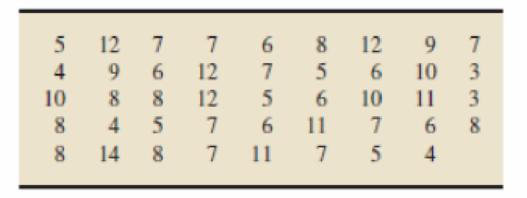
Cottonmouth Litter Size. In the article “The Eastern Cottonmouth (Agkistrodon piscivorus) at the Northern Edge of Its Range” (Journal of Herpetology, Vol. 29, No. 3, pp. 391–398), C. Blem and L. Blem examined the reproductive characteristics of the eastern cottonmouth, a once widely distributed snake whose numbers have decreased recently due to encroachment by humans. A simple random sample of 44 female cottonmouths yielded the following data on number of young per litter.

Chapter 8.1, Problem 18E, Cottonmouth Litter Size. In the article The Eastern Cottonmouth (Agkistrodon piscivorus) at the

a. Use the data to obtain a point estimate for the mean number of young per litter, μ, of all female eastern cottonmouths. (Note: ∑x_i = 334.)
b. Is your point estimate in part (a) likely to equal μ exactly? Explain your answer.

Definition Definition Measure of central tendency that is the average of a given data set. The mean value is evaluated as the quotient of the sum of all observations by the sample size. The mean, in contrast to a median, is affected by extreme values. Very large or very small values can distract the mean from the center of the data. Arithmetic mean: The most common type of mean is the arithmetic mean. It is evaluated using the formula: μ = 1 N ∑ i = 1 N x i Other types of means are the geometric mean, logarithmic mean, and harmonic mean. Geometric mean: The nth root of the product of n observations from a data set is defined as the geometric mean of the set: G = x 1 x 2 ... x n n Logarithmic mean: The difference of the natural logarithms of the two numbers, divided by the difference between the numbers is the logarithmic mean of the two numbers. The logarithmic mean is used particularly in heat transfer and mass transfer. ln x 2 − ln x 1 x 2 − x 1 Harmonic mean: The inverse of the arithmetic mean of the inverses of all the numbers in a data set is the harmonic mean of the data. 1 1 x 1 + 1 x 2 + ...

Expert Solution & Answer

Want to see the full answer?

Check out a sample textbook solution

See solution

Chapter 8.1, Problem 17E

Chapter 8.1, Problem 19E

Students have asked these similar questions

Ghost of Speciation Past. In the article, “Ghost of Speciation Past” (Nature, Vol. 435, pp. 29–31), T. Kocher looked at the origins of a diverse flock of cichlid fishes in the lakes of southeast Africa. Suppose that you wanted to select a sample from the hundreds of species of cichlid fishes that live in the lakes of southeast Africa. If you took a simple random sample from the species of each lake and combined all the simple random samples into one sample, which type of sampling design would you have used? Explain your answer.

1.7 Fisher's irises: Sir Ronald Aylmer Fisher was an English statistician, evolutionary biologist, and geneticist who worked on a data set that contained sepal length and width, and petal length and width from three species of iris flowers (setosa, versicolor and virginica). There were 58 flowers from each species in the data set. a) How many cases were included in the data? b) How many numerical variables are included in the data? Indicate what they are, and if they are continuous or discrete. Four continuous variables: sepal length, sepal width, petal length, and petal width Two discrete variables: sepal and petal Two continuous variables: length and width Four discrete variables: sepal length, sepal width, petal length, and petal width c) How many categorical variables are included in the data, and what are they? List the corresponding levels (categories). Three categorical variables: setosa, versicolor, and virginica Two categorical variables: species (levels: setosa,…

QUESTION 2 A researcher has conducted a sample survey about games addiction of secondary school students in certain district of country ABC. Luckily, it was found that only 20% of students were among the addicted students, even though total result from population study for the whole country of ABC showed that on average 80% of the secondary students were addicted. a) What is the population of interest? b) What is the sample? c) What is the value of parameter? d) What is the value of statistic?

Chapter 8 Solutions

Introductory Statistics (10th Edition)

Ch. 8.1 - The value of a statistic used to estimate a...Ch. 8.1 - What is a confidence-interval estimate of a...Ch. 8.1 - Prob. 3E Ch. 8.1 - Prob. 4E Ch. 8.1 - Prob. 5E Ch. 8.1 - Suppose that you lake 500 simple random samples...Ch. 8.1 - Prob. 7E Ch. 8.1 - A simple random sample is taken from a population...Ch. 8.1 - Refer to Exercise 8.7 and find a point estimate...Ch. 8.1 - Prob. 10E

Knowledge Booster

$Statistics$

Learn more about

Need a deep-dive on the concept behind this application? Look no further. Learn more about this topic, statistics and related others by exploring similar questions and additional content below.

Solution Summary: The author explains that the point estimate of the population mean number of young per litter is 7.591.

Concept explainers

Videos

Want to see the full answer?

Chapter 8 Solutions