Videos
a) Show that there are no critical points when
b) Find the critical point(s) and determine the eigenvalues of the associated Jacobian matrix when
c) How do you think trajectories of the system will behavefor
d) Choose one or two other initial points and plot the corresponding trajectories. Do these plots agree with your expectations?
(a)
To prove: There are no critical points for the system
Explanation of Solution
Given information:
The system of equations is
Formula used:
Quadratic formula:
The roots of the equations
Proof:
Consider
By plugging
The system becomes
The points, if any, where
The critical points of the system
Consider the first equation
Consider the second equation
Now plug these value in the equation
By using the quadratic formula,
Thus the value of
That is,
Thus there is no critical point when
Also, there are two distinct real values of when
That is,
Thus there are two critical points when
If
Thus there is only one critical point for the system.
(b)
The critical points of the system
Answer to Problem 1P
Solution:
When
When
Explanation of Solution
Given information:
The system is
Explanation:
The system is
By plugging
The system becomes,
From part (a),
The critical point is
Hence if
Therefore, the critical point is
Since
i) Near the critical point
To find eigenvalues of the matrix
Let
The characteristics equation is
Thus the eigenvalues when
The system is
By plugging
The system becomes,
From part (a),
The critical point is
Hence if
That is,
Therefore, the critical points are
Since
ii) Near the critical point
To find eigenvalues of the matrix
Let
The characteristics equation is
iii) Near the critical point
To find eigenvalues of the matrix
Let
The characteristics equation is
Thus the eigenvalues when
(c)
How the trajectories of the system will behave for
Answer to Problem 1P
Solution:
As
The trajectory starting at origin is:
The graph is agreeing with our expectations.
Explanation of Solution
Given information:
The system is
Explanation:
The system is
From part (b),
The eigenvalues corresponding to the critical point
Thus one of the eigenvalueshasa positive real part. Therefore, the critical point
The eigenvalues corresponding to the critical point
Thus the eigenvalues have a negative real part. Therefore, the critical point
Therefore, as
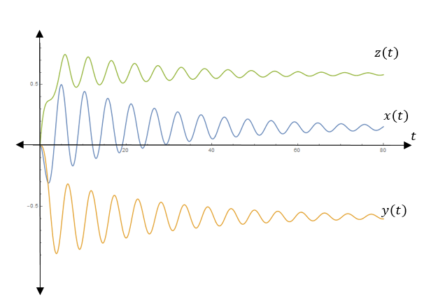
The trajectory starting at the origin is:
As
Therefore, the graph is agreeing with our expectations.
(d)
To graph: The corresponding trajectories by choosing one or two initial points. Whether these plots agree with your expectations or not.
Explanation of Solution
Given information:
The system is
Graph:
The trajectory with the initial condition
The trajectory with the initial condition
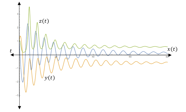
The trajectory with the initial point close to
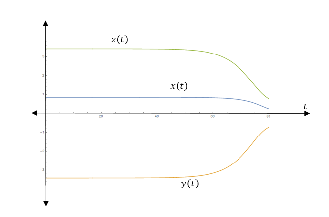
The trajectory with the initial point close to
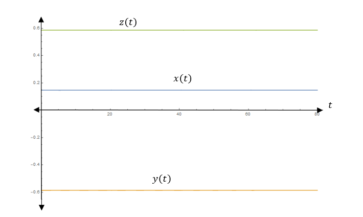
Interpretation:
From the above graph,
All trajectories converge to the point
From part (c),
As
Therefore, the graph agrees with our expectations.
Want to see more full solutions like this?
Chapter 7 Solutions
Differential Equations: An Introduction to Modern Methods and Applications
Additional Math Textbook Solutions
Using and Understanding Mathematics: A Quantitative Reasoning Approach (6th Edition)
University Calculus: Early Transcendentals (4th Edition)
Elementary Statistics: Picturing the World (7th Edition)
Elementary Statistics
Algebra and Trigonometry (6th Edition)
A First Course in Probability (10th Edition)


- Compare the interest earned from #1 (where simple interest was used) to #5 (where compound interest was used). The principal, annual interest rate, and time were all the same; the only difference was that for #5, interest was compounded quarterly. Does the difference in interest earned make sense? Select one of the following statements. a. No, because more money should have been earned through simple interest than compound interest. b. Yes, because more money was earned through simple interest. For simple interest you earn interest on interest, not just on the amount of principal. c. No, because more money was earned through simple interest. For simple interest you earn interest on interest, not just on the amount of principal. d. Yes, because more money was earned when compounded quarterly. For compound interest you earn interest on interest, not just on the amount of principal.arrow_forwardReduce the matrix to reduced row-echelon form. [3 2 -2-191 A = 3 -2 0 5 + 2 1 -2 -14 17 1 0 0 3 0 1 0 0 0 4arrow_forwardCompare and contrast the simple and compound interest formulas. Which one of the following statements is correct? a. Simple interest and compound interest formulas both yield principal plus interest, so you must subtract the principal to get the amount of interest. b. Simple interest formula yields principal plus interest, so you must subtract the principal to get the amount of interest; Compound interest formula yields only interest, which you must add to the principal to get the final amount. c. Simple interest formula yields only interest, which you must add to the principal to get the final amount; Compound interest formula yields principal plus interest, so you must subtract the principal to get the amount of interest. d. Simple interest and compound interest formulas both yield only interest, which you must add to the principal to get the final amount.arrow_forward
- Sara would like to go on a vacation in 5 years and she expects her total costs to be $3000. If she invests $2500 into a savings account for those 5 years at 8% interest, compounding semi-annually, how much money will she have? Round your answer to the nearest cent. Show you work. Will she be able to go on vacation? Why or why not?arrow_forwardIf $8000 is deposited into an account earning simple interest at an annual interest rate of 4% for 10 years, howmuch interest was earned? Show you work.arrow_forwardWhy is this proof incorrect? State what statement and/or reason is incorrect and why. Given: Overline OR is congruent to overline OQ, angle N is congruent to angle PProve: Angle 3 is congruent to angle 5 Why is this proof incorrect? Statements Reasons 1. Overline OR is congruent to overline OQ, angle N is congruent to angle P 1. Given 2. Overline ON is congruent to overline OP 2. Converse of the Isosceles Triangle Theorem 3. Triangle ONR is congruent to triangle OPQ 3. SAS 4. Angle 3 is congruent to angle 5 4. CPCTCarrow_forward
- x³-343 If k(x) = x-7 complete the table and use the results to find lim k(x). X-7 x 6.9 6.99 6.999 7.001 7.01 7.1 k(x) Complete the table. X 6.9 6.99 6.999 7.001 7.01 7.1 k(x) (Round to three decimal places as needed.)arrow_forward(3) (4 points) Given three vectors a, b, and c, suppose: |bx c = 2 |a|=√√8 • The angle between a and b xc is 0 = 135º. . Calculate the volume a (bxc) of the parallelepiped spanned by the three vectors.arrow_forwardCalculate these limits. If the limit is ∞ or -∞, write infinity or-infinity. If the limit does not exist, write DNE: Hint: Remember the first thing you check when you are looking at a limit of a quotient is the limit value of the denominator. 1. If the denominator does not go to 0, you should be able to right down the answer immediately. 2. If the denominator goes to 0, but the numerator does not, you will have to check the sign (±) of the quotient, from both sides if the limit is not one-sided. 3. If both the numerator and the denominator go to 0, you have to do the algebraic trick of rationalizing. So, group your limits into these three forms and work with them one group at a time. (a) lim t-pi/2 sint-√ sin 2t+14cos ² t 7 2 2 2cos t (b) lim sint + sin 2t+14cos = ∞ t-pi/2 2 2cos t (c) lim cost-√sin 2t+14cos² t = t-pi/2 2cos t (d) lim t→pi/2 cost+√ sin t + 14cos 2cos ² t = ∞ (e) lim sint-v sin 2 t + 14cos = 0 t-pi/2 (f) lim t-pi/2 sin t +√ sin 2sin 2 t 2 t + 14cos t 2sin t cost- (g)…arrow_forward
- Think of this sheet of paper as the plane containing the vectors a = (1,1,0) and b = (2,0,0). Sketch the parallelogram P spanned by a and b. Which diagonal of P represents the vector a--b geometrically?arrow_forwardGiven: AABE ~ ACDE. Prove: AC bisects BD. Note: quadrilateral properties are not permitted in this proof. Step Statement Reason AABE ACDE Given 2 ZDEC ZAEB Vertical angles are congruent try Type of Statement A E B D Carrow_forward10-2 Let A = 02-4 and b = 4 Denote the columns of A by a₁, a2, a3, and let W = Span {a1, a2, a̸3}. -4 6 5 - 35 a. Is b in {a1, a2, a3}? How many vectors are in {a₁, a₂, a3}? b. Is b in W? How many vectors are in W? c. Show that a2 is in W. [Hint: Row operations are unnecessary.] a. Is b in {a₁, a2, a3}? Select the correct choice below and, if necessary, fill in the answer box(es) to complete your choice. ○ A. No, b is not in {a₁, a2, 3} since it cannot be generated by a linear combination of a₁, a2, and a3. B. No, b is not in (a1, a2, a3} since b is not equal to a₁, a2, or a3. C. Yes, b is in (a1, a2, a3} since b = a (Type a whole number.) D. Yes, b is in (a1, a2, 3} since, although b is not equal to a₁, a2, or a3, it can be expressed as a linear combination of them. In particular, b = + + ☐ az. (Simplify your answers.)arrow_forward
 Algebra & Trigonometry with Analytic GeometryAlgebraISBN:9781133382119Author:SwokowskiPublisher:Cengage
 Linear Algebra: A Modern IntroductionAlgebraISBN:9781285463247Author:David PoolePublisher:Cengage Learning
 Elementary Linear Algebra (MindTap Course List)AlgebraISBN:9781305658004Author:Ron LarsonPublisher:Cengage Learning
 College Algebra (MindTap Course List)AlgebraISBN:9781305652231Author:R. David Gustafson, Jeff HughesPublisher:Cengage Learning