Concept explainers
Videos
Video Games and Grade-Point Average Professor Grant Alexander wanted to find a linear model that relates the number of hours a student plays video games each week. , to the cumulative grade-point average. , of the student. He obtained a random sample of 10 full-time students at his college and asked each student to disclose the number of hours spent playing video games and the student’s cumulative grade-point average.
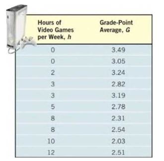
(a) Explain why the number of hours spent playing video games is the independent variable and cumulative grade-point average is the dependent variable.
(b) Use a graphing utility to draw a
(c) Use a graphing utility to find the line of best fit that models the relation between number of hours of video game playing each week and grade-point average. Express the model using function notation.
(d) Interpret the slope.
(e) Predict the grade-point average of a student who plays video games for 8 hours each week.
(f) How many hours of video game playing do you think a student plays whose grade-point average is ?
Want to see the full answer?
Check out a sample textbook solution
Chapter 3 Solutions
Precalculus Enhanced with Graphing Utilities, Books a la Carte Edition Plus NEW MyLab Math -- Access Card Package (7th Edition)


- Does Table 1 represent a linear function? If so, finda linear equation that models the data.arrow_forwardIf you travel 100 miles in two hours, then your average speed for the trip is Average speed=_________=________arrow_forwardThe table below shows the number of state-registered automatic weapons and the murder rate for several Northwestern states. X 11.3 y 13.3 10.9 9.9 8.4 6.8 3.9 2.8 2.4 2.5 7 6.7 6.4 6.3 x = thousands of automatic weapons y = murders per 100,000 residents This data can be modeled by the equation ŷ = 0.79x + 4.32. Use this equation to answer the following. Answer = 12.829 0.9 5 A) How many murders per 100,000 residents can be expected in a state with 10.1 thousand automatic weapons? Answer = 6.123 x Round to 3 decimal places. B) How many murders per 100,000 residents can be expected in a state with 2.7 thousand automatic weapons? x Round to 3 decimal places.arrow_forward
- Can subpoints d to f be explained pleasedarrow_forwardResearchers initiated a long-term study of the population of American black bears. One aspect of the study was to develop a model that could be used to predict a bear's weight (since it is not practical to weigh bears in the field). One variable thought to be related to weight is the length of the bear. The accompanying data represent the lengths and weights of 12 American black bears. Complete parts (a) through (d) below. Click the icon to view the data table. Click the icon to view the critical values table. ..... (a) Which variable is the explanatory variable based on the goals of the research? O A. The number of bears B. The weight of the bear O C. The length of the bear (b) Draw a scatter diagram of the data. Choose the correct graph below. O A. O B. O C. D. A Weight (kg) 180- AWeight (kg) 180- ALength (cm) 180- A Weight (kg) 180- 40- 100 40- 100 Length (cm) 40- 100 40- 100 200 200 200 200 Length (cm) Weight (kg) Length (cm) (c) Determine the linear correlation coefficient between…arrow_forwardA magazine publishes restaurant ratings for various locations around the world. The magazine rates the restaurants for food, decor, service, and the cost per person. Develop a regression model to predict the cost per person, based on a variable that represents the sum of the three ratings. The magazine has compiled the accompanying table of this summated ratings variable and the cost per person for 25 restaurants in a major city. Complete parts (a) through (e) below. Click the icon to view the table of summated ratings and cost per person. ..... a. Construct a scatter plot. Choose the correct graph below. A. Ов. С. D. ACost ($) 90- ACost ($) 90- ACost ($) 90- ACost ($) 90- 0- 0- 90 90 90 90 Rating Rating Rating Rating b. Assuming a linear relationship, use the least-squares method to compute the regression coefficients b, and b,. bo = and b, (Round to two decimal places as needed.) c. Interpret the meaning of the Y-intercept, bo, and the slope, b,. Choose the correct answer below. O A.…arrow_forward
- A magazine publishes restaurant ratings for various locations around the world. The magazine rates the restaurants for food, decor, service, and the cost per person. Develop a regression model to predict the cost per person, based on a variable that represents the sum of the three ratings. The magazine has compiled the accompanying table of this summated ratings variable and the cost per person for 25 restaurants in a major city. Complete parts (a) through (e) below. Click the icon to view the table of summated ratings and cost per person. a. Construct a scatter plot. Choose the correct graph below. O A. 90+ 0 0 Cost ($) The M Rating 90 Q O B. A Cost (5) 90+ 0 H +4 Alpe Rating 90 Q b. Assuming a linear relationship, use the least-squares method to compute the regression coefficients bo and b₁. bo= and b₁ = (Round to two decimal places as needed.) C O C. 90+ 0- Cost (S) HA Rating 90 Q Summated Ratings and Cost Per Person Summated Rating Cost ($ per person) 40 48 60 61 42 40 43 55 67 69…arrow_forwardA magazine publishes restaurant ratings for various locations around the world. The magazine rates the restaurants for food, decor, service, and the cost per person. Develop a regression model to predict the cost per person, based on a variable that represents the sum of the three ratings. The magazine has compiled the accompanying table of this summated ratings variable and the cost per person for 25 restaurants in a major city. Complete parts (a) through (e) below. Click the icon to view the table of summated ratings and cost per person. a. Construct a scatter plot. Choose the correct graph below. O A. Ов. OC. OD. ACost ($) 90- Q A Cost ($) 904 A Cost ($) 90- ACost ($) 90- 0- 0- 0- 0- 90 Rating 90 Rating 90 90 Rating Rating Summated ratings and cost per person b. Assuming a linear relationship, use the least-squares method to compute the regression coefficients bo and b,. bo =D and b, =O (Round to two decimal places as needed.) Summated Rating Cost ($ per person)|9 c. Interpret the…arrow_forwardA random sample of 136 adults were asked to report the number of hours per week the spent on a computer and their number of years of education. The linear model equation below describes the relationship between the mean computers hours and years of education. computers == 9.12 ++ 0.8 ×× education Based on this linear model, which of the following statements is correct? a) An adult who has no years of education is expected to spend 9.12 hours per week on a computer. b) An adult who has 1 more year of education than another is expected to spend 9.12 more hours per week on a computer. c) An adult who spends 1 more hour per week on a computer than another is expected to have had 9.12 more years of education. d) An adult who spend zero hours per week on a computer is expected to have 9.12 years of education.arrow_forward
- Q1: Please use the data set to create a regression equation or a regression line that can reflect the relationship between wealth and level of education in CA counties. NOTES: You are required to: 1) clearly state what is the dependent variable (Y) and what is the independent variable (X); 2) correctly calculate the associated slope and intercept. Q2: Please predict the related median household income when there is 70% of population over 25 with BA degree and higher. Median Household Income ($) % of population over 25 with BA degree and higher 100,929 42.1 71,348 20.5 59,961 25.0 69,588 21.1 108,689 39.4 90,996 32.1 63,284 19.5 53,746 27.5 58,528 13.4 66,834 15.2…arrow_forwardA medical statistician wanted to examine the relationship between the amount of sunshine (x) and incidence of skin cancer (y). As an experiment he found the number of skin cancers detected per 100,000 of population and the average daily sunshine in eight counties around the country. These data are shown below.Draw a scatter plot of the data and comment on the relationship between the 2 variables, predicting what the skin cancer rate might be for 10 hours of daily sunshine.arrow_forwardDraw a scatter diagram with square feet of living space as the independent variable and selling price as the dependent variable and describe variable and describe the relationship between the size of a house and the selling price.arrow_forward

 Glencoe Algebra 1, Student Edition, 9780079039897...AlgebraISBN:9780079039897Author:CarterPublisher:McGraw Hill
 Holt Mcdougal Larson Pre-algebra: Student Edition...AlgebraISBN:9780547587776Author:HOLT MCDOUGALPublisher:HOLT MCDOUGAL
 Big Ideas Math A Bridge To Success Algebra 1: Stu...AlgebraISBN:9781680331141Author:HOUGHTON MIFFLIN HARCOURTPublisher:Houghton Mifflin Harcourt
 College AlgebraAlgebraISBN:9781305115545Author:James Stewart, Lothar Redlin, Saleem WatsonPublisher:Cengage Learning