
Concept explainers
Videos
a.
To plot: The
Given information:
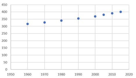
The atmospheric concentration of carbon dioxide (in parts per million) recorded by the observatory in years between 1960 and 2015.
| x | y |
| 1960 | 317 |
| 1970 | 326 |
| 1980 | 339 |
| 1990 | 354 |
| 2000 | 369 |
| 2005 | 380 |
| 2010 | 390 |
| 2015 | 401 |
Plot:
Take the year as x coordinate and concentration as y coordinate, and then draw the scatter plot as shown below:
Interpretation:
From the scatter plot it seems that the linear regression will best fit the scenario.
b.
To find: If a linear or a quadratic model fit more appropriate.
A linear model seems more appropriate for the scatter plot.
Given information:
The atmospheric concentration of carbon dioxide (in parts per million) recorded by the observatory in years between 1960 and 2015.
| x | y |
| 1960 | 317 |
| 1970 | 326 |
| 1980 | 339 |
| 1990 | 354 |
| 2000 | 369 |
| 2005 | 380 |
| 2010 | 390 |
| 2015 | 401 |
Calculation:
Observe that the points do not fall nearly along a well-known curve. But, they do seem to fall near a line with upward slope.
Since the curve drawn seems to be a straight line, a linear model seems more appropriate for the scatter plot.
c.
To find: Find the regression equation for the appropriate model, and superimpose the graph of the regression equation on the scatter plot.
The regression can line by written as
Given information:
The atmospheric concentration of carbon dioxide (in parts per million) recorded by the observatory in years between 1960 and 2015.
| x | y |
| 1960 | 317 |
| 1970 | 326 |
| 1980 | 339 |
| 1990 | 354 |
| 2000 | 369 |
| 2005 | 380 |
| 2010 | 390 |
| 2015 | 401 |
Calculation:
Prepare the table to find the regression coefficients as follows;
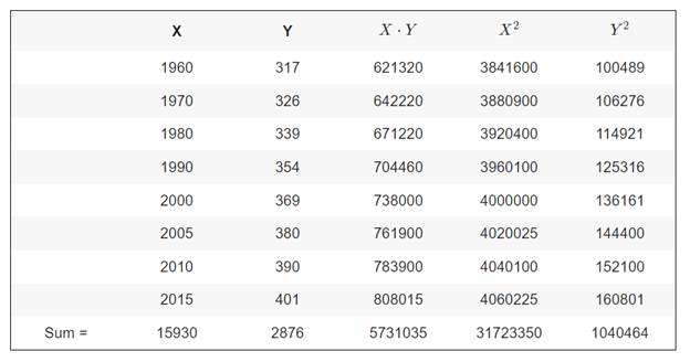
Use the table to perform the calculations as shown below.
Then,
Therefore,
So, the regression can line by written as
Now, plot the regression line as shown below.
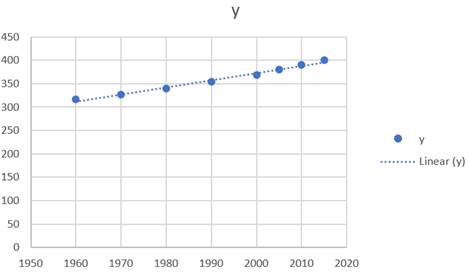
The graph of the regression line best fit the data. That means, the graph shows that the model appears to work well.
d.
To find: The approximate concentration level of carbon dioxide in the year 2025.
The concentration of carbon dioxide in the year 2025 will be
Given information:
The atmospheric concentration of carbon dioxide (in parts per million) recorded by the observatory in years between 1960 and 2015.
| x | y |
| 1960 | 317 |
| 1970 | 326 |
| 1980 | 339 |
| 1990 | 354 |
| 2000 | 369 |
| 2005 | 380 |
| 2010 | 390 |
| 2015 | 401 |
Calculation:
The model for the given situation is
Substitute
Conclusion:
The concentration of carbon dioxide in the year 2025 will be
e.
To explain: The circumstances that might caused the predication in part (d) of the mark and tell whether the true value will be higher or lower than the predicted value.
Given information:
The atmospheric concentration of carbon dioxide (in parts per million) recorded by the observatory in years between 1960 and 2015.
| x | y |
| 1960 | 317 |
| 1970 | 326 |
| 1980 | 339 |
| 1990 | 354 |
| 2000 | 369 |
| 2005 | 380 |
| 2010 | 390 |
| 2015 | 401 |
Explanation:
If the model is predicted to be an upward quadratic, then the prediction in part (d) would have been off the mark.
Since an upward quadratic function gives a higher value than a linear function with upward slope, the true value would have been lower than the predicated value.
Chapter 1 Solutions
PRECALCULUS:GRAPH...-NASTA ED.(FLORIDA)


- Under certain conditions, the number of diseased cells N(t) at time t increases at a rate N'(t) = Aekt, where A is the rate of increase at time 0 (in cells per day) and k is a constant. (a) Suppose A = 60, and at 3 days, the cells are growing at a rate of 180 per day. Find a formula for the number of cells after t days, given that 200 cells are present at t = 0. (b) Use your answer from part (a) to find the number of cells present after 8 days. (a) Find a formula for the number of cells, N(t), after t days. N(t) = (Round any numbers in exponents to five decimal places. Round all other numbers to the nearest tenth.)arrow_forwardThe marginal revenue (in thousands of dollars) from the sale of x handheld gaming devices is given by the following function. R'(x) = 4x (x² +26,000) 2 3 (a) Find the total revenue function if the revenue from 125 devices is $17,939. (b) How many devices must be sold for a revenue of at least $50,000? (a) The total revenue function is R(x) = (Round to the nearest integer as needed.) given that the revenue from 125 devices is $17,939.arrow_forwardUse substitution to find the indefinite integral. S 2u √u-4 -du Describe the most appropriate substitution case and the values of u and du. Select the correct choice below and fill in the answer boxes within your choice. A. Substitute u for the quantity in the numerator. Let v = , so that dv = ( ) du. B. Substitute u for the quantity under the root. Let v = u-4, so that dv = (1) du. C. Substitute u for the quantity in the denominator. Let v = Use the substitution to evaluate the integral. so that dv= ' ( du. 2u -du= √√u-4arrow_forward
- Use substitution to find the indefinite integral. Зи u-8 du Describe the most appropriate substitution case and the values of u and du. Select the correct choice below and fill in the answer boxes within your choice. A. Substitute u for the quantity in the numerator. Let v = , so that dv = ( ( ) du. B. Substitute u for the quantity under the root. Let v = u-8, so that dv = (1) du. C. Substitute u for the quantity in the denominator. Let v = so that dv= ( ) du. Use the substitution to evaluate the integral. S Зи -du= u-8arrow_forwardFind the derivative of the function. 5 1 6 p(x) = -24x 5 +15xarrow_forward∞ 2n (4n)! Let R be the radius of convergence of the series -x2n. Then the value of (3" (2n)!)² n=1 sin(2R+4/R) is -0.892 0.075 0.732 -0.812 -0.519 -0.107 -0.564 0.588arrow_forward
- Find the cost function if the marginal cost function is given by C'(x) = x C(x) = 2/5 + 5 and 32 units cost $261.arrow_forwardFind the cost function if the marginal cost function is C'(x) = 3x-4 and the fixed cost is $9. C(x) = ☐arrow_forwardFor the power series ∞ (−1)" (2n+1)(x+4)” calculate Z, defined as follows: n=0 (5 - 1)√n if the interval of convergence is (a, b), then Z = sin a + sin b if the interval of convergence is (a, b), then Z = cos asin b if the interval of convergence is (a, b], then Z = sin a + cos b if the interval of convergence is [a, b], then Z = cos a + cos b Then the value of Z is -0.502 0.117 -0.144 -0.405 0.604 0.721 -0.950 -0.588arrow_forward
- H-/ test the Series 1.12 7√2 by ratio best 2n 2-12- nz by vitio test enarrow_forwardHale / test the Series 1.12 7√2 2n by ratio best 2-12- nz by vico tio test en - プ n2 rook 31() by mood fest 4- E (^)" by root test Inn 5-E 3' b. E n n³ 2n by ratio test ٤ by Comera beon Test (n+2)!arrow_forwardEvaluate the double integral ' √ √ (−2xy² + 3ry) dA R where R = {(x,y)| 1 ≤ x ≤ 3, 2 ≤ y ≤ 4} Double Integral Plot of integrand and Region R N 120 100 80- 60- 40 20 -20 -40 2 T 3 4 5123456 This plot is an example of the function over region R. The region and function identified in your problem will be slightly different. Answer = Round your answer to four decimal places.arrow_forward
 Calculus: Early TranscendentalsCalculusISBN:9781285741550Author:James StewartPublisher:Cengage Learning
 Thomas' Calculus (14th Edition)CalculusISBN:9780134438986Author:Joel R. Hass, Christopher E. Heil, Maurice D. WeirPublisher:PEARSON
 Calculus: Early Transcendentals (3rd Edition)CalculusISBN:9780134763644Author:William L. Briggs, Lyle Cochran, Bernard Gillett, Eric SchulzPublisher:PEARSON
 Calculus: Early TranscendentalsCalculusISBN:9781319050740Author:Jon Rogawski, Colin Adams, Robert FranzosaPublisher:W. H. Freeman
 Calculus: Early Transcendental FunctionsCalculusISBN:9781337552516Author:Ron Larson, Bruce H. EdwardsPublisher:Cengage Learning