
Concept explainers
Videos
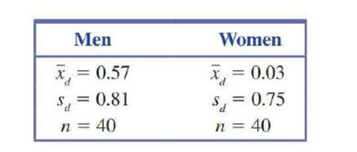
The paper “The Truth About Lying in Online Dating Profiles” (Proceedings, Computer-Human Interaction [2007]: 1–4) describes an investigation in which 40 men and 40 women with online dating profiles agreed to participate in a study. Each participant’s height (in inches) was measured and the actual height was compared to the height given in that person’s online profile. The differences between the online profile height and the actual height (profile – actual) were used to calculate the values in the accompanying table.
You can assume it is reasonable to regard the two samples in this study as being representative of male online daters and female online daters. (Although the authors of the paper believed that their samples were representative of these populations, participants were volunteers recruited through newspaper advertisements, so we should be a bit hesitant to generalize results to all online daters.)
- a. Use the paired t test to determine if there is convincing evidence that, on average, male online daters overstate their height in online dating profiles. Use α = 0.05.
- b. Construct and interpret a 95% confidence interval for the difference between the mean online dating profile height and mean actual height for female online daters. (Hint: See Example 11.8.)
- c. Use the two-sample t test of Section 11.1 to test H0: μm – μf = 0 versus Ha: μm – μf > 0, where μm is the mean height difference (profile – actual) for male online daters and μf, is the mean height difference (profile – actual) for female online daters.
- d. Explain why a paired t test was used in Part (a) but a two-sample t test was used in Part (c).
a.
Check whether there is convincing evidence that the average male online daters overstate their height in online dating profile or not.
Answer to Problem 29E
There is convincing evidence that the average male online daters overstate their height in online dating profile.
Explanation of Solution
Calculation:
Total of 40 men and 40 women are sampled. The sample size, standard deviation, and mean for diference between profile height and actual height, for men and women are given.
Assumption for conducting the test:
- The sample difference should be a random sample.
- The population distribution for the mean differences should follow approximately normal distribution.
- The samples are paired.
Here, the samples are paired. It is reasonable to assume that the two samples of men and women acts as the representative for all the male online daters and female online daters.
Let
Let
Here,
That is,
Hypotheses:
Null hypothesis:
That is, the mean difference between profile height and actual height, for men is zero.
Alternative hypothesis:
That is, the mean difference between profile height and actual height is greater than zero.
Test statistic:
Software procedure:
Step by step procedure to obtain the test statistic by using MINITAB software is given below:
- Choose Stat > Basic Statistics > Paired t.
- Choose summarized data.
- In choose sample size as 40, means as 0.57 and standard deviation as 0.81.
- Choose Options.
- In Confidence level, enter 95.
- In Alternative, select greater than.
- Click OK in all dialogue boxes.
Output using the MINITAB software is given below:
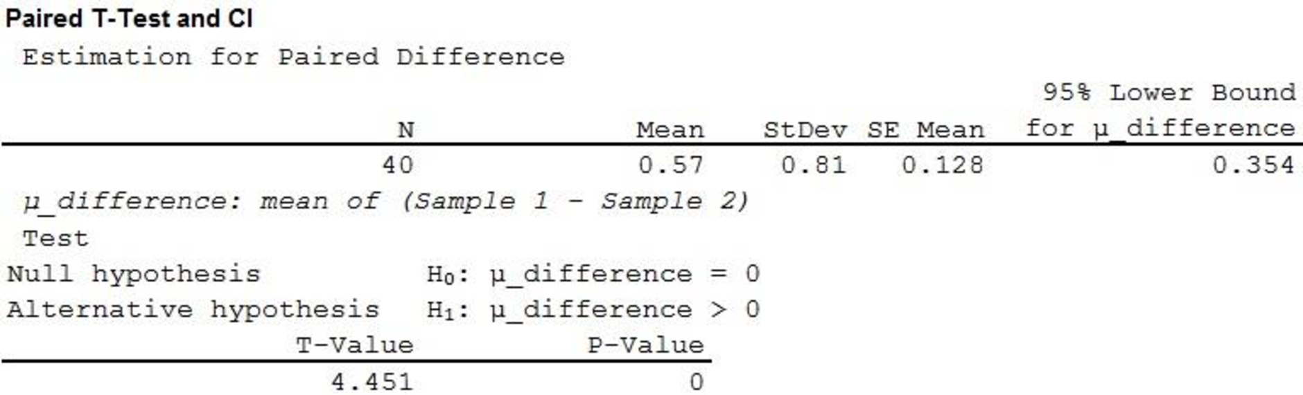
From the above MINITAB output the test statistic is 4.451 and the P-value is 0.
Decision rule:
- If P-value is less than or equal to the level of significance, reject the null hypothesis.
- Otherwise fail to reject the null hypothesis.
Conclusion:
Here, the level of significance is 0.05.
Here, P-value is less than the level of significance.
That is,
Therefore, reject the null hypothesis.
It can be concluded that there is convincing evidence that the average male online daters overstate their height in online dating profile.
b.
Construct a 95% confidence interval for the difference in mean profile height and mean actual height for female online daters.
Interpret the interval.
Answer to Problem 29E
The 95% confidence interval for the difference in mean profile height and mean actual height for female online daters is
Explanation of Solution
Calculation:
Assumptions for conducting the hypothesis test:
- The sample difference should be a random sample.
- The population distribution for the mean differences should follow approximately normal distribution.
- The samples are paired.
Here, samples are paired. The selected samples were representatives of population. Since the sample size is large
Confidence interval:
Software procedure:
Step by step procedure to obtain the confidence interval by using MINITAB software is as follows:
- Choose Stat > Basic Statistics > Paired t.
- Choose summarized data.
- In choose sample size as 40, means as 0.03 and standard deviation as 0.75.
- Choose Options.
- In Confidence level, enter 95.
- In Alternative, select not equal.
- Click OK in all dialogue boxes.
Output using the MINITAB software is given below:
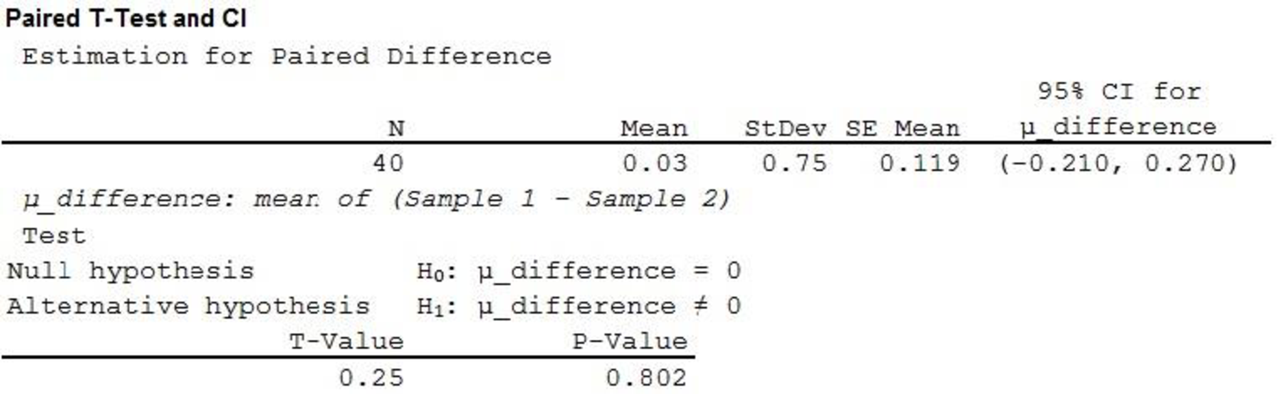
From the output, the 95% confidence interval is
Interpretation:
One can be 95% confident that the difference in mean profile height and mean actual height for female online daters lies between –0.210 and 0.270.
c.
Conduct a two sample t-test.
Answer to Problem 29E
There is convincing evidence that the mean height difference is higher for males than females.
Explanation of Solution
Calculation:
In this context, two sample t-test is used for the comparison.
Assumption for the two sample t-test:
- The random samples should be collected independently.
- The sample sizes should be large. That is, each sample size is at least 30. Or the populations are approximately normally distributed.
Requirement check:
Here, samples are selected at random from the population. Each sample has size of 40, which is greater than 30.
Therefore, the assumptions are satisfied.
Let
Let
Hypotheses:
Null hypothesis:
That is, the mean height difference is same for both males and females.
Alternative hypothesis:
That is, the mean height difference is higher for males than females.
Test statistic and P-value:
Software procedure:
Step by step procedure to obtain the P-value and test statistic by using MINITAB software:
- Choose Stat > Basic Statistics > 2 sample t.
- Choose Summarized data.
- In sample 1, enter Sample size as 40, Mean as 0.57, Standard deviation as 0.03.
- In sample 2, enter Sample size as 40, Mean as 0.03, Standard deviation as 0.75.
- Choose Options.
- In Confidence level, enter 95.
- In Alternative, select greater than.
- Click OK in all the dialogue boxes.
Output using the MINITAB software is given below:
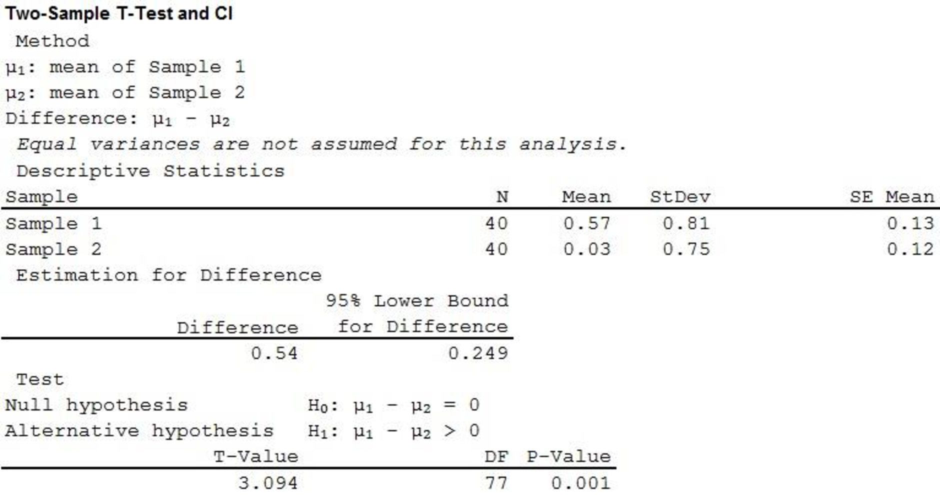
Therefore, the P-value is 0.001 and the test statistic is 3.094.
Decision rule:
- If P-value is less than or equal to the level of significance, reject the null hypothesis.
- Otherwise fail to reject the null hypothesis.
Conclusion:
Here, the level of significance is 0.05.
Here, P-value is less than the level of significance.
That is,
Therefore, reject the null hypothesis.
Hence, it can be concluded that there is convincing evidence that the mean height difference is higher for males than females.
d.
Explain the reason for paired t test was used in Part (a) two sample t-test was used in Part (c).
Explanation of Solution
Calculation:
In this context, the result obtained in Part (a) compares the mean actual and profile height for males. That is, the male profile and actual heights are paired. Therefore, the paired t test was used in Part (a).
Now, in this case, the result obtained in Part (c) compares the mean height difference for male and female. That is, the samples of male and female are independent. Therefore, the two sample t-test was used in Part (c).
Want to see more full solutions like this?
Chapter 11 Solutions
Introduction to Statistics and Data Analysis


- You find out that the dietary scale you use each day is off by a factor of 2 ounces (over — at least that’s what you say!). The margin of error for your scale was plus or minus 0.5 ounces before you found this out. What’s the margin of error now?arrow_forwardSuppose that Sue and Bill each make a confidence interval out of the same data set, but Sue wants a confidence level of 80 percent compared to Bill’s 90 percent. How do their margins of error compare?arrow_forwardSuppose that you conduct a study twice, and the second time you use four times as many people as you did the first time. How does the change affect your margin of error? (Assume the other components remain constant.)arrow_forward
- Out of a sample of 200 babysitters, 70 percent are girls, and 30 percent are guys. What’s the margin of error for the percentage of female babysitters? Assume 95 percent confidence.What’s the margin of error for the percentage of male babysitters? Assume 95 percent confidence.arrow_forwardYou sample 100 fish in Pond A at the fish hatchery and find that they average 5.5 inches with a standard deviation of 1 inch. Your sample of 100 fish from Pond B has the same mean, but the standard deviation is 2 inches. How do the margins of error compare? (Assume the confidence levels are the same.)arrow_forwardA survey of 1,000 dental patients produces 450 people who floss their teeth adequately. What’s the margin of error for this result? Assume 90 percent confidence.arrow_forward
- The annual aggregate claim amount of an insurer follows a compound Poisson distribution with parameter 1,000. Individual claim amounts follow a Gamma distribution with shape parameter a = 750 and rate parameter λ = 0.25. 1. Generate 20,000 simulated aggregate claim values for the insurer, using a random number generator seed of 955.Display the first five simulated claim values in your answer script using the R function head(). 2. Plot the empirical density function of the simulated aggregate claim values from Question 1, setting the x-axis range from 2,600,000 to 3,300,000 and the y-axis range from 0 to 0.0000045. 3. Suggest a suitable distribution, including its parameters, that approximates the simulated aggregate claim values from Question 1. 4. Generate 20,000 values from your suggested distribution in Question 3 using a random number generator seed of 955. Use the R function head() to display the first five generated values in your answer script. 5. Plot the empirical density…arrow_forwardFind binomial probability if: x = 8, n = 10, p = 0.7 x= 3, n=5, p = 0.3 x = 4, n=7, p = 0.6 Quality Control: A factory produces light bulbs with a 2% defect rate. If a random sample of 20 bulbs is tested, what is the probability that exactly 2 bulbs are defective? (hint: p=2% or 0.02; x =2, n=20; use the same logic for the following problems) Marketing Campaign: A marketing company sends out 1,000 promotional emails. The probability of any email being opened is 0.15. What is the probability that exactly 150 emails will be opened? (hint: total emails or n=1000, x =150) Customer Satisfaction: A survey shows that 70% of customers are satisfied with a new product. Out of 10 randomly selected customers, what is the probability that at least 8 are satisfied? (hint: One of the keyword in this question is “at least 8”, it is not “exactly 8”, the correct formula for this should be = 1- (binom.dist(7, 10, 0.7, TRUE)). The part in the princess will give you the probability of seven and less than…arrow_forwardplease answer these questionsarrow_forward
- Selon une économiste d’une société financière, les dépenses moyennes pour « meubles et appareils de maison » ont été moins importantes pour les ménages de la région de Montréal, que celles de la région de Québec. Un échantillon aléatoire de 14 ménages pour la région de Montréal et de 16 ménages pour la région Québec est tiré et donne les données suivantes, en ce qui a trait aux dépenses pour ce secteur d’activité économique. On suppose que les données de chaque population sont distribuées selon une loi normale. Nous sommes intéressé à connaitre si les variances des populations sont égales.a) Faites le test d’hypothèse sur deux variances approprié au seuil de signification de 1 %. Inclure les informations suivantes : i. Hypothèse / Identification des populationsii. Valeur(s) critique(s) de Fiii. Règle de décisioniv. Valeur du rapport Fv. Décision et conclusion b) A partir des résultats obtenus en a), est-ce que l’hypothèse d’égalité des variances pour cette…arrow_forwardAccording to an economist from a financial company, the average expenditures on "furniture and household appliances" have been lower for households in the Montreal area than those in the Quebec region. A random sample of 14 households from the Montreal region and 16 households from the Quebec region was taken, providing the following data regarding expenditures in this economic sector. It is assumed that the data from each population are distributed normally. We are interested in knowing if the variances of the populations are equal. a) Perform the appropriate hypothesis test on two variances at a significance level of 1%. Include the following information: i. Hypothesis / Identification of populations ii. Critical F-value(s) iii. Decision rule iv. F-ratio value v. Decision and conclusion b) Based on the results obtained in a), is the hypothesis of equal variances for this socio-economic characteristic measured in these two populations upheld? c) Based on the results obtained in a),…arrow_forwardA major company in the Montreal area, offering a range of engineering services from project preparation to construction execution, and industrial project management, wants to ensure that the individuals who are responsible for project cost estimation and bid preparation demonstrate a certain uniformity in their estimates. The head of civil engineering and municipal services decided to structure an experimental plan to detect if there could be significant differences in project evaluation. Seven projects were selected, each of which had to be evaluated by each of the two estimators, with the order of the projects submitted being random. The obtained estimates are presented in the table below. a) Complete the table above by calculating: i. The differences (A-B) ii. The sum of the differences iii. The mean of the differences iv. The standard deviation of the differences b) What is the value of the t-statistic? c) What is the critical t-value for this test at a significance level of 1%?…arrow_forward
 Glencoe Algebra 1, Student Edition, 9780079039897...AlgebraISBN:9780079039897Author:CarterPublisher:McGraw Hill
 Big Ideas Math A Bridge To Success Algebra 1: Stu...AlgebraISBN:9781680331141Author:HOUGHTON MIFFLIN HARCOURTPublisher:Houghton Mifflin Harcourt
 College Algebra (MindTap Course List)AlgebraISBN:9781305652231Author:R. David Gustafson, Jeff HughesPublisher:Cengage Learning
 Holt Mcdougal Larson Pre-algebra: Student Edition...AlgebraISBN:9780547587776Author:HOLT MCDOUGALPublisher:HOLT MCDOUGAL