
Videos
a.
Check whether the data provide convincing support for the claim that, on average, male teenager drivers exceed the speed limit by more than do female teenage drivers.
a.
Answer to Problem 18E
The conclusion is that the data provide convincing support for the claim that, on average, male teenager drivers exceed the speed limit by more than do female teenage drivers.
Explanation of Solution
Calculation:
The data are based on the speed limit for male and female drivers.
Step 1:
In this context,
Step 2:
Null hypothesis:
Step 3:
Alternative hypothesis:
Step 4:
Significance level,
It is given that the significance level,
Step 5:
Test statistic:
Step 6:
The assumption for the two-sample t-test:
- The random samples should be collected independently.
- The sample sizes should be large. That is, each sample size is at least 30 or the populations are approximately normally distributed.
It is assumed that the distribution of the speed limit for male and female drivers is normally distributed.
Boxplot:
Software procedure:
Step-by-step procedure to obtain a boxplot using MINITAB software:
- Choose Graphs > Boxplot.
- Under Multiple Y’s, choose Simple.
- In Graph variables, enter the column of Male Driver and Female Driver.
- In Scale, choose Transpose values and categorical scales.
- Click OK in all dialogue boxes.
Output using MINITAB software is given below:
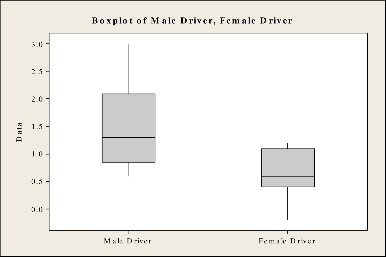
Any lack of symmetric that appears in the boxplot is acceptable for the given sample size because the sample size is larger.
From the boxplot, it is clear that the distribution of the speed limit for male drivers is skewed right and the distribution of the speed limit for female drivers is skewed left. Based on the sample size, the normality condition is satisfied. Morevoer, random samples are collected independently. Therefore, the assumptions are satisfied. It is reasonable to use the data for a two-sample t test.
Step 7:
Test statistic:
Software procedure:
Step-by-step procedure to obtain the P-value and test statistic using MINITAB software:
- Choose Stat > Basic Statistics > 2 sample t.
- Choose Samples in different columns.
- In sample 1, enter the column of Male Driver.
- In sample 2, enter the column of Female Driver.
- Choose Options.
- In Confidence level, enter 95.
- In Alternative, select greater than.
- Click OK in all the dialogue boxes.
Output obtained using MINITAB software is given below:
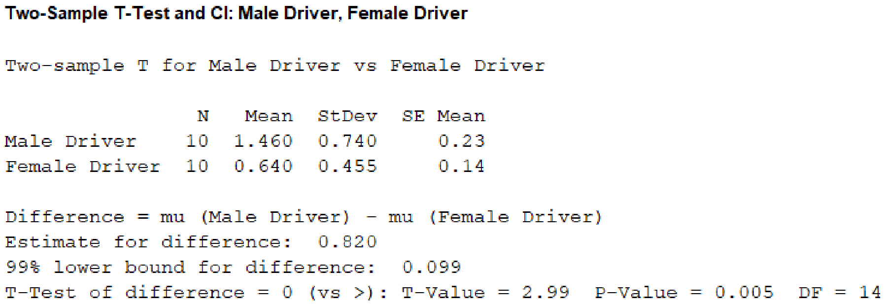
From the given MINITAB output, the value of the test statistic is 2.99.
Step 8:
P-value:
From the MINITAB output, the P-value is 0.005.
Step 9:
Decision rule:
If the
Here, the
That is,
The decision is that the null hypothesis is rejected.
Conclusion:
Hence, the data provide convincing support for the claim that, on average, male teenager drivers exceed the speed limit by more than do female teenage drivers.
b.
(i)
Check whether there is sufficient evidence to conclude that the average number of miles per hour over the speed limit is greater for male drivers with male passengers than it is for male drivers with female passengers.
(ii)
Check whether there is sufficient evidence to conclude that the average number of miles per hour over the speed limit is greater for female drivers with male passengers than it is for female drivers with female passengers.
(iii)
Check whether there is sufficient evidence to conclude that the average number of miles per hour over the speed limit is smaller for male drivers with female passengers than it is for female drivers with male passengers.
b.
Answer to Problem 18E
(i)
The conclusion is that there is sufficient evidence to conclude that the average number of miles per hour over the speed limit is greater for male drivers with male passengers than it is for male drivers with female passengers.
(ii)
The conclusion is that there is sufficient evidence to conclude that the average number of miles per hour over the speed limit is greater for female drivers with male passengers than it is for female drivers with female passengers.
(iii)
The conclusion is that there is sufficient evidence to conclude that the average number of miles per hour over the speed limit is smaller for male drivers with female passengers than it is for female drivers with male passengers.
Explanation of Solution
Calculation:
(i)
Step 1:
In this context,
Step 2:
Null hypothesis:
Step 3:
Alternative hypothesis:
Step 4:
Significance level,
It is given that the significance level
Step 5:
Test statistic:
Step 6:
Assumptions for the two-sample t-test:
- The random samples should be collected independently.
- The sample sizes should be large. That is, each sample size must be at least 30.
Assumption in this particular problem:
- Data are collected independently.
- The sample sizes are large.
Here, both sample sizes are greater than 30.
Therefore, the assumptions are satisfied.
Step 7:
Test statistic:
Software procedure:
Step-by-step procedure to obtain the P-value and test statistic using MINITAB software:
- Choose Stat > Basic Statistics > 2 sample t.
- Choose Summarized data.
- In sample 1, enter Sample size as 40, Mean as 5.2, Standard deviation as 0.8.
- In sample 2, enter Sample size as 40, Mean as 0.3, Standard deviation as 0.8.
- Choose Options.
- In Confidence level, enter 99.
- In Alternative, select greater than.
- Click OK in all the dialogue boxes.
Output obtained using MINITAB software is given below:
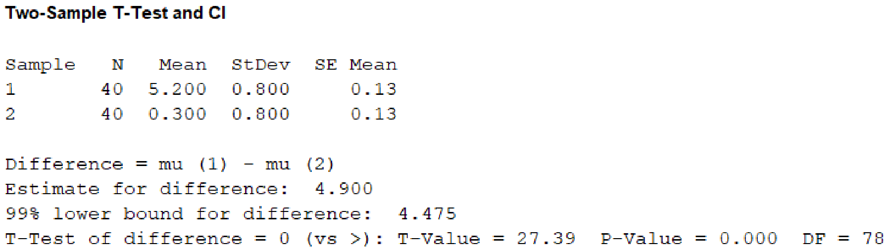
From the given MINITAB output, the value of test statistic is 27.39.
Step 8:
P-value:
From the MINITAB output, the P-value is 0.
Step 9:
Decision rule:
If the
Here, the
That is,
The decision is that the null hypothesis is rejected.
Conclusion:
Hence, there is sufficient evidence to conclude that the average number of miles per hour over the speed limit is greater for male drivers with male passengers than it is for male drivers with female passengers.
(ii)
Step 1:
In this context,
Step 2:
Null hypothesis:
Step 3:
Alternative hypothesis:
Step 4:
Significance level,
It is given that the significance level
Step 5:
Test statistic:
Step 6:
Assumptions for the two-sample t-test:
- The random samples should be collected independently.
- The sample sizes should be large. That is, each sample size must be at least 30.
Assumption in this particular problem:
- Data are collected independently.
- The sample sizes are large.
Here, both sample sizes are greater than 30.
Therefore, the assumptions are satisfied.
Step 7:
Test statistic:
Software procedure:
Step-by-step procedure to obtain the P-value and test statistic using MINITAB software:
- Choose Stat > Basic Statistics > 2 sample t.
- Choose Summarized data.
- In sample 1, enter Sample size as 40, Mean as 2.3, Standard deviation as 0.8.
- In sample 2, enter Sample size as 40, Mean as 0.6, Standard deviation as 0.8.
- Choose Options.
- In Confidence level, enter 99.
- In Alternative, select greater than.
- Click OK in all the dialogue boxes.
Output obtained using MINITAB software is given below:
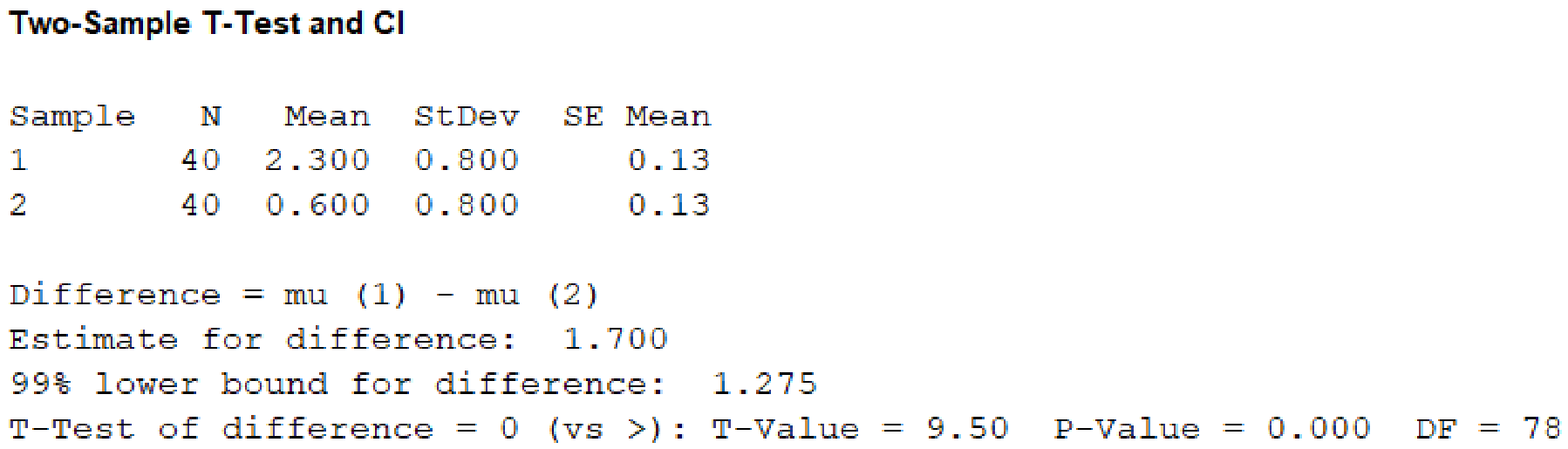
From the given MINITAB output, the value of test statistic is 9.50.
Step 8:
P-value:
From the MINITAB output, the P-value is 0.
Step 9:
Decision rule:
If the
Here, the
That is,
The decision is that the null hypothesis is rejected.
Conclusion:
Hence, there is sufficient evidence to conclude that the average number of miles per hour over the speed limit is greater for female drivers with male passengers than it is for female drivers with female passengers.
(iii)
Step 1:
In this context,
Step 2:
Null hypothesis:
Step 3:
Alternative hypothesis:
Step 4:
Significance level,
It is given that the significance level
Step 5:
Test statistic:
Step 6:
Assumptions for the two-sample t-test:
- The random samples should be collected independently.
- The sample sizes should be large. That is, each sample size must be at least 30.
Assumption in this particular problem:
- Data are collected independently.
- The sample sizes are large.
Here, both sample sizes are greater than 30.
Therefore, the assumptions are satisfied.
Step 7:
Test statistic:
Software procedure:
Step-by-step procedure to obtain the P-value and test statistic using MINITAB software:
- Choose Stat > Basic Statistics > 2 sample t.
- Choose Summarized data.
- In sample 1, enter Sample size as 40, Mean as 0.3, Standard deviation as 0.8.
- In sample 2, enter Sample size as 40, Mean as 2.3, Standard deviation as 0.8.
- Choose Options.
- In Confidence level, enter 99.
- In Alternative, select less than.
- Click OK in all the dialogue boxes.
Output obtained using the MINITAB software is given below:
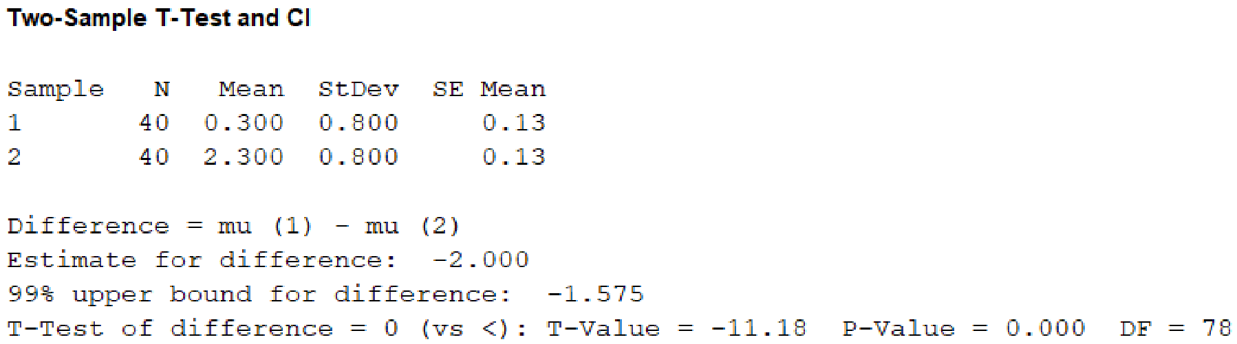
From the given MINITAB output, the value of test statistic is –11.18.
Step 8:
P-value:
From the MINITAB output, the P-value is 0.
Step 9:
Decision rule:
If the
Here, the
That is,
The decision is that the null hypothesis is rejected.
Conclusion:
Hence, there is sufficient evidence to conclude that the average number of miles per hour over the speed limit is smaller for male drivers with female passengers than it is for female drivers with male passengers.
c.
Comment on the effects of gender on teenagers driving with passengers.
c.
Explanation of Solution
Comment:
From the results, it is observed that the average speed limit for male and female drivers are greater with male passengers when compared to the female passengers. The average speed limit for male drivers are lesser with female passengers when compared to the female drivers with male passengers. The average speed limit for male drivers are greater with male passengers when compared to the female drivers with female passengers.
Want to see more full solutions like this?
Chapter 11 Solutions
Introduction to Statistics and Data Analysis


- a) Let X and Y be independent random variables both with the same mean µ=0. Define a new random variable W = aX +bY, where a and b are constants. (i) Obtain an expression for E(W).arrow_forwardThe table below shows the estimated effects for a logistic regression model with squamous cell esophageal cancer (Y = 1, yes; Y = 0, no) as the response. Smoking status (S) equals 1 for at least one pack per day and 0 otherwise, alcohol consumption (A) equals the average number of alcohoic drinks consumed per day, and race (R) equals 1 for blacks and 0 for whites. Variable Effect (β) P-value Intercept -7.00 <0.01 Alcohol use 0.10 0.03 Smoking 1.20 <0.01 Race 0.30 0.02 Race × smoking 0.20 0.04 Write-out the prediction equation (i.e., the logistic regression model) when R = 0 and again when R = 1. Find the fitted Y S conditional odds ratio in each case. Next, write-out the logistic regression model when S = 0 and again when S = 1. Find the fitted Y R conditional odds ratio in each case.arrow_forwardThe chi-squared goodness-of-fit test can be used to test if data comes from a specific continuous distribution by binning the data to make it categorical. Using the OpenIntro Statistics county_complete dataset, test the hypothesis that the persons_per_household 2019 values come from a normal distribution with mean and standard deviation equal to that variable's mean and standard deviation. Use signficance level a = 0.01. In your solution you should 1. Formulate the hypotheses 2. Fill in this table Range (-⁰⁰, 2.34] (2.34, 2.81] (2.81, 3.27] (3.27,00) Observed 802 Expected 854.2 The first row has been filled in. That should give you a hint for how to calculate the expected frequencies. Remember that the expected frequencies are calculated under the assumption that the null hypothesis is true. FYI, the bounderies for each range were obtained using JASP's drag-and-drop cut function with 8 levels. Then some of the groups were merged. 3. Check any conditions required by the chi-squared…arrow_forward
- Suppose that you want to estimate the mean monthly gross income of all households in your local community. You decide to estimate this population parameter by calling 150 randomly selected residents and asking each individual to report the household’s monthly income. Assume that you use the local phone directory as the frame in selecting the households to be included in your sample. What are some possible sources of error that might arise in your effort to estimate the population mean?arrow_forwardFor the distribution shown, match the letter to the measure of central tendency. A B C C Drag each of the letters into the appropriate measure of central tendency. Mean C Median A Mode Barrow_forwardA physician who has a group of 38 female patients aged 18 to 24 on a special diet wishes to estimate the effect of the diet on total serum cholesterol. For this group, their average serum cholesterol is 188.4 (measured in mg/100mL). Suppose that the total serum cholesterol measurements are normally distributed with standard deviation of 40.7. (a) Find a 95% confidence interval of the mean serum cholesterol of patients on the special diet.arrow_forward
- The accompanying data represent the weights (in grams) of a simple random sample of 10 M&M plain candies. Determine the shape of the distribution of weights of M&Ms by drawing a frequency histogram. Find the mean and median. Which measure of central tendency better describes the weight of a plain M&M? Click the icon to view the candy weight data. Draw a frequency histogram. Choose the correct graph below. ○ A. ○ C. Frequency Weight of Plain M and Ms 0.78 0.84 Frequency OONAG 0.78 B. 0.9 0.96 Weight (grams) Weight of Plain M and Ms 0.84 0.9 0.96 Weight (grams) ○ D. Candy Weights 0.85 0.79 0.85 0.89 0.94 0.86 0.91 0.86 0.87 0.87 - Frequency ☑ Frequency 67200 0.78 → Weight of Plain M and Ms 0.9 0.96 0.84 Weight (grams) Weight of Plain M and Ms 0.78 0.84 Weight (grams) 0.9 0.96 →arrow_forwardThe acidity or alkalinity of a solution is measured using pH. A pH less than 7 is acidic; a pH greater than 7 is alkaline. The accompanying data represent the pH in samples of bottled water and tap water. Complete parts (a) and (b). Click the icon to view the data table. (a) Determine the mean, median, and mode pH for each type of water. Comment on the differences between the two water types. Select the correct choice below and fill in any answer boxes in your choice. A. For tap water, the mean pH is (Round to three decimal places as needed.) B. The mean does not exist. Data table Тар 7.64 7.45 7.45 7.10 7.46 7.50 7.68 7.69 7.56 7.46 7.52 7.46 5.15 5.09 5.31 5.20 4.78 5.23 Bottled 5.52 5.31 5.13 5.31 5.21 5.24 - ☑arrow_forwardく Chapter 5-Section 1 Homework X MindTap - Cengage Learning x + C webassign.net/web/Student/Assignment-Responses/submit?pos=3&dep=36701632&tags=autosave #question3874894_3 M Gmail 品 YouTube Maps 5. [-/20 Points] DETAILS MY NOTES BBUNDERSTAT12 5.1.020. ☆ B Verify it's you Finish update: All Bookmarks PRACTICE ANOTHER A computer repair shop has two work centers. The first center examines the computer to see what is wrong, and the second center repairs the computer. Let x₁ and x2 be random variables representing the lengths of time in minutes to examine a computer (✗₁) and to repair a computer (x2). Assume x and x, are independent random variables. Long-term history has shown the following times. 01 Examine computer, x₁₁ = 29.6 minutes; σ₁ = 8.1 minutes Repair computer, X2: μ₂ = 92.5 minutes; σ2 = 14.5 minutes (a) Let W = x₁ + x2 be a random variable representing the total time to examine and repair the computer. Compute the mean, variance, and standard deviation of W. (Round your answers…arrow_forward
- The acidity or alkalinity of a solution is measured using pH. A pH less than 7 is acidic; a pH greater than 7 is alkaline. The accompanying data represent the pH in samples of bottled water and tap water. Complete parts (a) and (b). Click the icon to view the data table. (a) Determine the mean, median, and mode pH for each type of water. Comment on the differences between the two water types. Select the correct choice below and fill in any answer boxes in your choice. A. For tap water, the mean pH is (Round to three decimal places as needed.) B. The mean does not exist. Data table Тар Bottled 7.64 7.45 7.46 7.50 7.68 7.45 7.10 7.56 7.46 7.52 5.15 5.09 5.31 5.20 4.78 5.52 5.31 5.13 5.31 5.21 7.69 7.46 5.23 5.24 Print Done - ☑arrow_forwardThe median for the given set of six ordered data values is 29.5. 9 12 23 41 49 What is the missing value? The missing value is ☐.arrow_forwardFind the population mean or sample mean as indicated. Sample: 22, 18, 9, 6, 15 □ Select the correct choice below and fill in the answer box to complete your choice. O A. x= B. μεarrow_forward
 Glencoe Algebra 1, Student Edition, 9780079039897...AlgebraISBN:9780079039897Author:CarterPublisher:McGraw Hill
 Big Ideas Math A Bridge To Success Algebra 1: Stu...AlgebraISBN:9781680331141Author:HOUGHTON MIFFLIN HARCOURTPublisher:Houghton Mifflin Harcourt
 College Algebra (MindTap Course List)AlgebraISBN:9781305652231Author:R. David Gustafson, Jeff HughesPublisher:Cengage Learning
 Holt Mcdougal Larson Pre-algebra: Student Edition...AlgebraISBN:9780547587776Author:HOLT MCDOUGALPublisher:HOLT MCDOUGAL