
Videos
Here’s one to sink your teeth into: The authors of the article “Analysis of Food Crushing Sounds During Mastication: Total Sound Level Studies” (Journal of Texture Studies [1990]: 165–178) studied the nature of sounds generated during eating. Peak loudness (in decibels at 20 cm away) was measured for both open-mouth and closed-mouth chewing of potato chips and of tortilla chips. Forty subjects participated, with ten assigned at random to each combination of conditions (such as closed-mouth potato chip, and so on). We are not making this up! Summary values taken from plots given in the article appear in the accompanying table. For purposes of this exercise, suppose that it is reasonable to regard the peak loudness distributions as approximately normal.
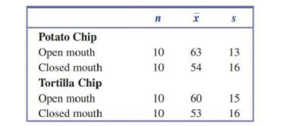
- a. Construct a 95% confidence interval tor the (inference in
mean peak loudness between open-mouth and closed-mouth chewing of potato chips. Interpret the resulting interval. - b. For closed-mouth chewing (the recommended method!), is there sufficient evidence to indicate that there is a difference between potato chips and tortilla chips with respect to mean peak loudness? Test the relevant hypotheses using α = 0.01.
- c. The means and standard deviations given here were actually for stale chips. When ten measurements of peak loudness were recorded for closed-mouth chewing of fresh tortilla chips, the resulting mean and standard deviation were 56 and 14, respectively. Is there sufficient evidence to conclude that chewing fresh tortilla chips is louder than chewing stale chips? Use α = 0.05.

Trending nowThis is a popular solution!

Chapter 11 Solutions
Introduction to Statistics and Data Analysis


- to complete the Case × T Civil Service Numerical Test Sec x T Casework Skills Practice Test + Vaseline euauthoring.panpowered.com/DeliveryWeb/Civil Service Main/84589a48-b934-4b6e-a6e1-a5d75f559df9?transferToken=MxNewOS NGFSPSZSMOMzuz The table below shows the best price available for various items from 4 uniform suppliers. The prices do not include VAT (charged at 20%). Item A1-Uniforms (£)Best Trade (£)Clothing Tech (£)Dress Right (£) Waterproof boots 59.99 39.99 59.99 49.99 Trousers 9.89 9.98 9.99 11.99 Shirts 14.99 15.99 16.99 12.99 Hi-Vis vest 4.49 4.50 4.00 4.00 20.00 25.00 19.50 19.99 Hard hats A company needs to buy a set of 12 uniforms which includes 1 of each item. If the special offers are included, which supplier is cheapest? O O O O A1-Uniforms Best Trade Clothing Tech Dress Right Q Search ENG L UK +0 F6 四吧 6 78 ㄓ F10 9% * CO 1 F12 34 Oarrow_forwardCritics review films out of 5 based on three attributes: the story, the special effects and the acting. The ratings of four critics for a film are collected in the table below.CriticSpecialStory rating Effects rating Acting rating Critic 14.44.34.5Critic 24.14.23.9Critic 33.943.4Critic 44.24.14.2Critic 1 also gave the film a rating for the Director's ability. If the average of Critic 1's ratings was 4.3 what rating did they give to the Director's ability?3.94.04.14.24.3arrow_forwardTwo measurements are made of some quantity. For the first measurement, the average is 74.4528, the RMS error is 6.7441, and the uncertainty of the mean is 0.9264. For the second one, the average is 76.8415, the standard deviation is 8.3348, and the uncertainty of the mean is 1.1448. The expected value is exactly 75. 13. Express the first measurement in public notation. 14. Is there a significant difference between the two measurements? 1 15. How does the first measurement compare with the expected value? 16. How does the second measurement compare with the expected value?arrow_forward
- A hat contains slips of paper numbered 1 through 6. You draw two slips of paper at random from the hat,without replacing the first slip into the hat.(a) (5 points) Write out the sample space S for this experiment.(b) (5 points) Express the event E : {the sum of the numbers on the slips of paper is 4} as a subset of S.(c) (5 points) Find P(E)(d) (5 points) Let F = {the larger minus the smaller number is 0}. What is P(F )?(e) (5 points) Are E and F disjoint? Why or why not?(f) (5 points) Find P(E ∪ F )arrow_forwardIn addition to the in-school milk supplement program, the nurse would like to increase the use of daily vitamin supplements for the children by visiting homes and educating about the merits of vitamins. She believes that currently, about 50% of families with school-age children give the children a daily megavitamin. She would like to increase this to 70%. She plans a two-group study, where one group serves as a control and the other group receives her visits. How many families should she expect to visit to have 80% power of detecting this difference? Assume that drop-out rate is 5%.arrow_forwardA recent survey of 400 americans asked whether or not parents do too much for their young adult children. The results of the survey are shown in the data file. a) Construct the frequency and relative frequency distributions. How many respondents felt that parents do too much for their adult children? What proportion of respondents felt that parents do too little for their adult children? b) Construct a pie chart. Summarize the findingsarrow_forward
- The average number of minutes Americans commute to work is 27.7 minutes (Sterling's Best Places, April 13, 2012). The average commute time in minutes for 48 cities are as follows: Click on the datafile logo to reference the data. DATA file Albuquerque 23.3 Jacksonville 26.2 Phoenix 28.3 Atlanta 28.3 Kansas City 23.4 Pittsburgh 25.0 Austin 24.6 Las Vegas 28.4 Portland 26.4 Baltimore 32.1 Little Rock 20.1 Providence 23.6 Boston 31.7 Los Angeles 32.2 Richmond 23.4 Charlotte 25.8 Louisville 21.4 Sacramento 25.8 Chicago 38.1 Memphis 23.8 Salt Lake City 20.2 Cincinnati 24.9 Miami 30.7 San Antonio 26.1 Cleveland 26.8 Milwaukee 24.8 San Diego 24.8 Columbus 23.4 Minneapolis 23.6 San Francisco 32.6 Dallas 28.5 Nashville 25.3 San Jose 28.5 Denver 28.1 New Orleans 31.7 Seattle 27.3 Detroit 29.3 New York 43.8 St. Louis 26.8 El Paso 24.4 Oklahoma City 22.0 Tucson 24.0 Fresno 23.0 Orlando 27.1 Tulsa 20.1 Indianapolis 24.8 Philadelphia 34.2 Washington, D.C. 32.8 a. What is the mean commute time for…arrow_forwardMorningstar tracks the total return for a large number of mutual funds. The following table shows the total return and the number of funds for four categories of mutual funds. Click on the datafile logo to reference the data. DATA file Type of Fund Domestic Equity Number of Funds Total Return (%) 9191 4.65 International Equity 2621 18.15 Hybrid 1419 2900 11.36 6.75 Specialty Stock a. Using the number of funds as weights, compute the weighted average total return for these mutual funds. (to 2 decimals) % b. Is there any difficulty associated with using the "number of funds" as the weights in computing the weighted average total return in part (a)? Discuss. What else might be used for weights? The input in the box below will not be graded, but may be reviewed and considered by your instructor. c. Suppose you invested $10,000 in this group of mutual funds and diversified the investment by placing $2000 in Domestic Equity funds, $4000 in International Equity funds, $3000 in Specialty Stock…arrow_forwardThe days to maturity for a sample of five money market funds are shown here. The dollar amounts invested in the funds are provided. Days to Maturity 20 Dollar Value ($ millions) 20 12 30 7 10 5 6 15 10 Use the weighted mean to determine the mean number of days to maturity for dollars invested in these five money market funds (to 1 decimal). daysarrow_forward
- c. What are the first and third quartiles? First Quartiles (to 1 decimals) Third Quartiles (to 4 decimals) × ☑ Which companies spend the most money on advertising? Business Insider maintains a list of the top-spending companies. In 2014, Procter & Gamble spent more than any other company, a whopping $5 billion. In second place was Comcast, which spent $3.08 billion (Business Insider website, December 2014). The top 12 companies and the amount each spent on advertising in billions of dollars are as follows. Click on the datafile logo to reference the data. DATA file Company Procter & Gamble Comcast Advertising ($billions) $5.00 3.08 2.91 Company American Express General Motors Advertising ($billions) $2.19 2.15 ETET AT&T Ford Verizon L'Oreal 2.56 2.44 2.34 Toyota Fiat Chrysler Walt Disney Company J.P Morgan a. What is the mean amount spent on advertising? (to 2 decimals) 2.55 b. What is the median amount spent on advertising? (to 3 decimals) 2.09 1.97 1.96 1.88arrow_forwardMartinez Auto Supplies has retail stores located in eight cities in California. The price they charge for a particular product in each city are vary because of differing competitive conditions. For instance, the price they charge for a case of a popular brand of motor oil in each city follows. Also shown are the number of cases that Martinez Auto sold last quarter in each city. City Price ($) Sales (cases) Bakersfield 34.99 501 Los Angeles 38.99 1425 Modesto 36.00 294 Oakland 33.59 882 Sacramento 40.99 715 San Diego 38.59 1088 San Francisco 39.59 1644 San Jose 37.99 819 Compute the average sales price per case for this product during the last quarter? Round your answer to two decimal places.arrow_forwardConsider the following data and corresponding weights. xi Weight(wi) 3.2 6 2.0 3 2.5 2 5.0 8 a. Compute the weighted mean (to 2 decimals). b. Compute the sample mean of the four data values without weighting. Note the difference in the results provided by the two computations (to 3 decimals).arrow_forward
 Glencoe Algebra 1, Student Edition, 9780079039897...AlgebraISBN:9780079039897Author:CarterPublisher:McGraw Hill