Control Systems Engineering
7th Edition
ISBN: 9781118170519
Author: Norman S. Nise
Publisher: WILEY
expand_more
expand_more
format_list_bulleted
Concept explainers
Videos
Textbook Question
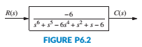
Chapter 6, Problem 6P
Determine how many closed-loop poles lie in the right half-plane. In the left half-plane, and on the
6. How many poles are in the tight half-plane, in the left half-plane, and on the
Expert Solution & Answer
Want to see the full answer?
Check out a sample textbook solution
Students have asked these similar questions
Practise question need help on
Can you show explaination and working. The answer from the text book is Q=5.03 X 10^-3
practise question
Chapter 6 Solutions
Control Systems Engineering
Ch. 6 - Prob. 1RQCh. 6 - Prob. 2RQCh. 6 - What would happen to a physical system chat...Ch. 6 - Why are marginally stable systems considered...Ch. 6 - Prob. 5RQCh. 6 - Prob. 6RQCh. 6 - Prob. 7RQCh. 6 - Prob. 8RQCh. 6 - Prob. 9RQCh. 6 - Why do we sometimes multiply a row of a Routh...
Ch. 6 - Prob. 11RQCh. 6 - Prob. 12RQCh. 6 - 13. Does the presence of an entire row of zeros...Ch. 6 - Prob. 14RQCh. 6 - Prob. 15RQCh. 6 - Prob. 16RQCh. 6 - Tell how many roots of the following polynomial...Ch. 6 - Tell how many roots of the following polynomial...Ch. 6 - Using the Routh table, tell how many poles of the...Ch. 6 - Prob. 4PCh. 6 - Determine how many closed-loop poles lie in the...Ch. 6 - Determine how many closed-loop poles lie in the...Ch. 6 - MATLAB ML 7. Use MATLAB to find the pole location...Ch. 6 - Symbolic Math SM 8. Use MATLAB and the Symbolic...Ch. 6 - Determine whether the unity feedback system of...Ch. 6 - Use MATLAB to find the pole locations for the...Ch. 6 - Consider the unity feedback system of Figure P6.3...Ch. 6 - In the system of Figure P6.3, let Gs=Ks+1ss2s+3...Ch. 6 - Given the unity feedback system of Figure P6.3...Ch. 6 - Using the Routh-Hurwitz criterion and the unity...Ch. 6 - Given the unity feedback system of Figure P6.3...Ch. 6 - Repeat Problem 15 using MATLAB.Ch. 6 - Prob. 17PCh. 6 - For the system of Figure P6.4, tell how many...Ch. 6 - Using the Routh-Hurwitz criterion, tell how many...Ch. 6 - Determine if the unity feedback system of Figure...Ch. 6 - For the unity feedback system of Figure P6.3 with...Ch. 6 - In the system of Figure P6.3, let Gs=Ksassb Find...Ch. 6 - For the unity feedback system of Figure P63 with...Ch. 6 - Find the range of K for stability for the unity...Ch. 6 - For the unity feedback system of Figure P6.3 with...Ch. 6 - find the range of K for stability. [Section: 6.41]...Ch. 6 - Find the range of gain, K, to ensure stability in...Ch. 6 - Using the Routh-Hurwitz criterion, find the value...Ch. 6 - Use the Routh-Hurwitz criterion to find the range...Ch. 6 - Prob. 32PCh. 6 - Given the unity feedback system of Figure P63 with...Ch. 6 - Repeat Problem 33 for [Section: 6.4]...Ch. 6 - For the system shown in Figure P6.8, find the...Ch. 6 - Given the unity feedback system of Figure P6.3...Ch. 6 - For the unity feedback system of Figure P6.3 with...Ch. 6 - For the unity feedback system of Figure P6.3 with...Ch. 6 - Given the unity feedback system of Figure P6.3...Ch. 6 - Using the Routh-Hurwitz criterion and the unity...Ch. 6 - Find the range of K to keep the system shown in...Ch. 6 - Prob. 43PCh. 6 - The closed-loop transfer function of a system is...Ch. 6 - Prob. 45PCh. 6 - Prob. 46PCh. 6 - An interval polynomial is of the form...Ch. 6 - A linearized model of a torque-controlled crane...Ch. 6 - The read/write head assembly arm of a computer...Ch. 6 - A system is represented in state space as...Ch. 6 - State Space SS 52. The following system in state...Ch. 6 - Prob. 54PCh. 6 - A model for an airplane’s pitch loop is shown in...Ch. 6 - Prob. 57PCh. 6 - Prob. 58PCh. 6 - Prob. 59PCh. 6 - Prob. 60PCh. 6 - Prob. 61PCh. 6 - Look-ahead information can be used to...Ch. 6 - Prob. 63PCh. 6 - It has been shown (Pounds, 2011) that an unloaded...Ch. 6 - Prob. 65PCh. 6 - The system shown in Figure P6.16 has G1s=1/ss+2s+4...Ch. 6 - Prob. 67PCh. 6 - Prob. 68PCh. 6 - Hybrid vehicle. Figure P6.l8 shows the HEV system...Ch. 6 - Prob. 70P
Knowledge Booster


Learn more about
Need a deep-dive on the concept behind this application? Look no further. Learn more about this topic, mechanical-engineering and related others by exploring similar questions and additional content below.Similar questions
- Can you provide steps and an explaination on how the height value to calculate the Pressure at point B is (-5-3.5) and the solution is 86.4kPa.arrow_forwardPROBLEM 3.46 The solid cylindrical rod BC of length L = 600 mm is attached to the rigid lever AB of length a = 380 mm and to the support at C. When a 500 N force P is applied at A, design specifications require that the displacement of A not exceed 25 mm when a 500 N force P is applied at A For the material indicated determine the required diameter of the rod. Aluminium: Tall = 65 MPa, G = 27 GPa. Aarrow_forwardFind the equivalent mass of the rocker arm assembly with respect to the x coordinate. k₁ mi m2 k₁arrow_forward
- 2. Figure below shows a U-tube manometer open at both ends and containing a column of liquid mercury of length l and specific weight y. Considering a small displacement x of the manometer meniscus from its equilibrium position (or datum), determine the equivalent spring constant associated with the restoring force. Datum Area, Aarrow_forward1. The consequences of a head-on collision of two automobiles can be studied by considering the impact of the automobile on a barrier, as shown in figure below. Construct a mathematical model (i.e., draw the diagram) by considering the masses of the automobile body, engine, transmission, and suspension and the elasticity of the bumpers, radiator, sheet metal body, driveline, and engine mounts.arrow_forward3.) 15.40 – Collar B moves up at constant velocity vB = 1.5 m/s. Rod AB has length = 1.2 m. The incline is at angle = 25°. Compute an expression for the angular velocity of rod AB, ė and the velocity of end A of the rod (✓✓) as a function of v₂,1,0,0. Then compute numerical answers for ȧ & y_ with 0 = 50°.arrow_forward
- 2.) 15.12 The assembly shown consists of the straight rod ABC which passes through and is welded to the grectangular plate DEFH. The assembly rotates about the axis AC with a constant angular velocity of 9 rad/s. Knowing that the motion when viewed from C is counterclockwise, determine the velocity and acceleration of corner F.arrow_forward500 Q3: The attachment shown in Fig.3 is made of 1040 HR. The static force is 30 kN. Specify the weldment (give the pattern, electrode number, type of weld, length of weld, and leg size). Fig. 3 All dimension in mm 30 kN 100 (10 Marks)arrow_forward(read image) (answer given)arrow_forward
- A cylinder and a disk are used as pulleys, as shown in the figure. Using the data given in the figure, if a body of mass m = 3 kg is released from rest after falling a height h 1.5 m, find: a) The velocity of the body. b) The angular velocity of the disk. c) The number of revolutions the cylinder has made. T₁ F Rd = 0.2 m md = 2 kg T T₂1 Rc = 0.4 m mc = 5 kg ☐ m = 3 kgarrow_forward(read image) (answer given)arrow_forward11-5. Compute all the dimensional changes for the steel bar when subjected to the loads shown. The proportional limit of the steel is 230 MPa. 265 kN 100 mm 600 kN 25 mm thickness X Z 600 kN 450 mm E=207×103 MPa; μ= 0.25 265 kNarrow_forward
arrow_back_ios
SEE MORE QUESTIONS
arrow_forward_ios
Recommended textbooks for you
 Elements Of ElectromagneticsMechanical EngineeringISBN:9780190698614Author:Sadiku, Matthew N. O.Publisher:Oxford University Press
 Mechanics of Materials (10th Edition)Mechanical EngineeringISBN:9780134319650Author:Russell C. HibbelerPublisher:PEARSON
 Thermodynamics: An Engineering ApproachMechanical EngineeringISBN:9781259822674Author:Yunus A. Cengel Dr., Michael A. BolesPublisher:McGraw-Hill Education
 Control Systems EngineeringMechanical EngineeringISBN:9781118170519Author:Norman S. NisePublisher:WILEY
 Mechanics of Materials (MindTap Course List)Mechanical EngineeringISBN:9781337093347Author:Barry J. Goodno, James M. GerePublisher:Cengage Learning
 Engineering Mechanics: StaticsMechanical EngineeringISBN:9781118807330Author:James L. Meriam, L. G. Kraige, J. N. BoltonPublisher:WILEY
Elements Of Electromagnetics
Mechanical Engineering
ISBN:9780190698614
Author:Sadiku, Matthew N. O.
Publisher:Oxford University Press
Mechanics of Materials (10th Edition)
Mechanical Engineering
ISBN:9780134319650
Author:Russell C. Hibbeler
Publisher:PEARSON
Thermodynamics: An Engineering Approach
Mechanical Engineering
ISBN:9781259822674
Author:Yunus A. Cengel Dr., Michael A. Boles
Publisher:McGraw-Hill Education
Control Systems Engineering
Mechanical Engineering
ISBN:9781118170519
Author:Norman S. Nise
Publisher:WILEY
Mechanics of Materials (MindTap Course List)
Mechanical Engineering
ISBN:9781337093347
Author:Barry J. Goodno, James M. Gere
Publisher:Cengage Learning
Engineering Mechanics: Statics
Mechanical Engineering
ISBN:9781118807330
Author:James L. Meriam, L. G. Kraige, J. N. Bolton
Publisher:WILEY
Introduction to Undamped Free Vibration of SDOF (1/2) - Structural Dynamics; Author: structurefree;https://www.youtube.com/watch?v=BkgzEdDlU78;License: Standard Youtube License