Concept explainers
Videos
a.
To calculate the coefficients
a.
Answer to Problem 66E
Explanation of Solution
Given information:
Quadratic approximation to
With the properties
Calculation :
Write the function and get the values at
Therefore,
b.
To find the quadratic approximation to
b.
Answer to Problem 66E
The quadratic approximation is
Explanation of Solution
Given information:
The given statement is that find the quadratic approximation to
Calculation :
Substitute the values in
Therefore,
The quadratic approximation is
c.
To graph:
c.
Explanation of Solution
Given information:
ZOOM IN on the two graphs at point
Graph:
The graph of
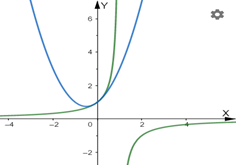
The image of ZOOM IN at point
Interpretation:
At the point
d.
To find the quadratic approximation to
d.
Answer to Problem 66E
The quadratic approximation is
The function and its approximation behave similar around
Explanation of Solution
Given information:
The given statement is that find the quadratic approximation to
Calculation :
Substitute the values in quadratic approximation equation
Therefore,
The quadratic approximation is
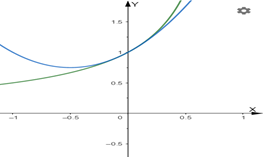
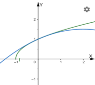
The graph of g and its quadratic approximation together.
The function and its approximation behave similar around
e.
To find the quadratic approximation to
e.
Answer to Problem 66E
The quadratic approximation is
The function and its approximation behave similar around
Explanation of Solution
Given information:
The given statement is that find the quadratic approximation to
Calculation :
Substitute the values in quadratic approximation equation
Therefore,
The quadratic approximation is
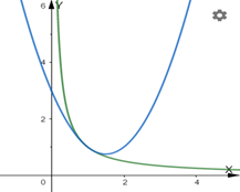
The graph of h and its quadratic approximation together.
The function and its approximation behave similar around
f.
To write the linearization of f , g , and h at the respective points.
f.
Answer to Problem 66E
Linearization of f , g , and h are
Explanation of Solution
Given information:
Functions are given in parts (b), (d), and (e)
Formula used:
Linearization.
Calculation :
For f
Linearization.
For g
Linearization.
For h
Linearization.
Therefore,
Linearization of f , g , and h are
Chapter 5 Solutions
Calculus: Graphical, Numerical, Algebraic
Additional Math Textbook Solutions
Elementary Statistics: Picturing the World (7th Edition)
A Problem Solving Approach To Mathematics For Elementary School Teachers (13th Edition)
Elementary Statistics
University Calculus: Early Transcendentals (4th Edition)
College Algebra (7th Edition)
Calculus: Early Transcendentals (2nd Edition)


- The spread of an infectious disease is often modeled using the following autonomous differential equation: dI - - BI(N − I) − MI, dt where I is the number of infected people, N is the total size of the population being modeled, ẞ is a constant determining the rate of transmission, and μ is the rate at which people recover from infection. Close a) (5 points) Suppose ẞ = 0.01, N = 1000, and µ = 2. Find all equilibria. b) (5 points) For the equilbria in part a), determine whether each is stable or unstable. c) (3 points) Suppose ƒ(I) = d. Draw a phase plot of f against I. (You can use Wolfram Alpha or Desmos to plot the function, or draw the dt function by hand.) Identify the equilibria as stable or unstable in the graph. d) (2 points) Explain the biological meaning of these equilibria being stable or unstable.arrow_forwardFind the indefinite integral. Check Answer: 7x 4 + 1x dxarrow_forwardshow sketcharrow_forward
- Find the indefinite integral. Check Answer: 7x 4 + 1x dxarrow_forwardQuestion 1: Evaluate the following indefinite integrals. a) (5 points) sin(2x) 1 + cos² (x) dx b) (5 points) t(2t+5)³ dt c) (5 points) √ (In(v²)+1) 4 -dv ขarrow_forwardFind the indefinite integral. Check Answer: In(5x) dx xarrow_forward
- Find the indefinite integral. Check Answer: 7x 4 + 1x dxarrow_forwardHere is a region R in Quadrant I. y 2.0 T 1.5 1.0 0.5 0.0 + 55 0.0 0.5 1.0 1.5 2.0 X It is bounded by y = x¹/3, y = 1, and x = 0. We want to evaluate this double integral. ONLY ONE order of integration will work. Good luck! The dA =???arrow_forward43–46. Directions of change Consider the following functions f and points P. Sketch the xy-plane showing P and the level curve through P. Indicate (as in Figure 15.52) the directions of maximum increase, maximum decrease, and no change for f. ■ 45. f(x, y) = x² + xy + y² + 7; P(−3, 3)arrow_forward
 Calculus: Early TranscendentalsCalculusISBN:9781285741550Author:James StewartPublisher:Cengage Learning
 Thomas' Calculus (14th Edition)CalculusISBN:9780134438986Author:Joel R. Hass, Christopher E. Heil, Maurice D. WeirPublisher:PEARSON
 Calculus: Early Transcendentals (3rd Edition)CalculusISBN:9780134763644Author:William L. Briggs, Lyle Cochran, Bernard Gillett, Eric SchulzPublisher:PEARSON
 Calculus: Early TranscendentalsCalculusISBN:9781319050740Author:Jon Rogawski, Colin Adams, Robert FranzosaPublisher:W. H. Freeman
 Calculus: Early Transcendental FunctionsCalculusISBN:9781337552516Author:Ron Larson, Bruce H. EdwardsPublisher:Cengage Learning