Calculus: Graphical, Numerical, Algebraic

3rd Edition

ISBN: 9780133688399

Author: Finney, Ross L.

Publisher: Pearson/Prentice Hall

See similar textbooks

Concept explainers

Differential Equations

Have you ever observed the movement of the satellites and rockets or how the planets go around the sun in their orbits? How will you determine their motion? Definitely they follow some scientific laws and these kinds of problems are framed as differentia…

Videos

Question

Chapter 5.3, Problem 32E

To determine

To find: the logistic regression for the data.

Expert Solution

Answer to Problem 32E

S=28984386.596891+49.25205e−0.85116t .

Explanation of Solution

Given information: Table shows the cumulative number of subscriber added to tat.

baseline number from 1978 to 1985.

Year since 1977	Added Subscribers Since 1977
1	1,391,910
2	2,814,380
3	5,671,490
4	11,219,200
5	17,340,570
6	22,113,790
7	25,290,870
8	27,872,520

Calculation:

The logistic regression curve, for number of subscriber S at t years after 1977 as produced by graphing utility:

S=28984386.596891+49.25205e−0.85116t .

To determine

To graph: the data in a scatter plot and super impose the regression curve.

Expert Solution

Answer to Problem 32E

Explanation of Solution

Given information: S=28984386.596891+49.25205e−0.85116t

Calculation:

Scatter plot of the table data with S=28984386.596891+49.25205e−0.85116t shown below.

Calculus: Graphical, Numerical, Algebraic, Chapter 5.3, Problem 32E , additional homework tip 1

To determine

To find: in what year between 1977 and 1985 were basic cable TV subscriptions growing the fastest and what significant behavior does the graph of the regression equation exhibit at that point .

Expert Solution

Answer to Problem 32E

Between 1981 and 1982.

Explanation of Solution

Given information: S=28984386.596891+49.25205e−0.85116t

Calculation:

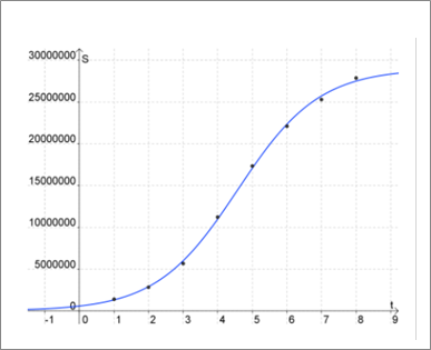
Scatter plot of the table data with S=28984386.596891+49.25205e−0.85116t shown below.

Calculus: Graphical, Numerical, Algebraic, Chapter 5.3, Problem 32E , additional homework tip 2

From the graph, the number of subscribers is increasing the fastest around t = 4 and t = 5 or between the year 1981 and 1982.

The slope of the tangent line at that point is greatest there, in other words, the change in the number of subscribers over the change in time is largest.

The concavity also changes at that point, so it is a point of inflection.

To determine

To find: what does the regression equation indicate about the number of basic cable television subscribers in the long run.

Expert Solution

Answer to Problem 32E

In the long term, the equation says the number of subscribers will stabilize at around

29 million.

Explanation of Solution

Given information: S=28984386.596891+49.25205e−0.85116t .

Calculation:

limt→∞28984386.596891+49.25205e−0.85116t=28984386.596891+49.25205e−0.85116(0)=28984386.59689≈29 million.

So, in the long term, the equation says the number of subscribers will stabilize at around 29 million.

To determine

Expert Solution

Answer to Problem 32E

To find: what circumstances changes to render the earlier model so ineffective.

Explanation of Solution

Given information: S=28984386.596891+49.25205e−0.85116t .

Calculation:

In the latter half of the 1990s, the cable companies heavily invested in and upgraded their networks, spreading out to more areas, installing fiber optics and stuff, increasing their ability to provide broadband internet and other services. These fitted curves don't usually work too much beyond the given data set anyway.

Chapter 5.3, Problem 31E

Chapter 5.3, Problem 33E

Chapter 5 Solutions

Calculus: Graphical, Numerical, Algebraic

Ch. 5.1 - Prob. 1QR Ch. 5.1 - Prob. 2QR Ch. 5.1 - Prob. 3QR Ch. 5.1 - Prob. 4QR Ch. 5.1 - Prob. 5QR Ch. 5.1 - Prob. 6QR Ch. 5.1 - Prob. 7QR Ch. 5.1 - Prob. 8QR Ch. 5.1 - Prob. 9QR Ch. 5.1 - Prob. 10QR

Ch. 5.1 - Prob. 11QR Ch. 5.1 - Prob. 12QR Ch. 5.1 - Prob. 1E Ch. 5.1 - Prob. 2E Ch. 5.1 - Prob. 3E Ch. 5.1 - Prob. 4E Ch. 5.1 - Prob. 5E Ch. 5.1 - Prob. 6E Ch. 5.1 - Prob. 7E Ch. 5.1 - Prob. 8E Ch. 5.1 - Prob. 9E Ch. 5.1 - Prob. 10E Ch. 5.1 - Prob. 11E Ch. 5.1 - Prob. 12E Ch. 5.1 - Prob. 13E Ch. 5.1 - Prob. 14E Ch. 5.1 - Prob. 15E Ch. 5.1 - Prob. 16E Ch. 5.1 - Prob. 17E Ch. 5.1 - Prob. 18E Ch. 5.1 - Prob. 19E Ch. 5.1 - Prob. 20E Ch. 5.1 - Prob. 21E Ch. 5.1 - Prob. 22E Ch. 5.1 - Prob. 23E Ch. 5.1 - Prob. 24E Ch. 5.1 - Prob. 25E Ch. 5.1 - Prob. 26E Ch. 5.1 - Prob. 27E Ch. 5.1 - Prob. 28E Ch. 5.1 - Prob. 29E Ch. 5.1 - Prob. 30E Ch. 5.1 - Prob. 31E Ch. 5.1 - Prob. 32E Ch. 5.1 - Prob. 33E Ch. 5.1 - Prob. 34E Ch. 5.1 - Prob. 35E Ch. 5.1 - Prob. 36E Ch. 5.1 - Prob. 37E Ch. 5.1 - Prob. 38E Ch. 5.1 - Prob. 39E Ch. 5.1 - Prob. 40E Ch. 5.1 - Prob. 41E Ch. 5.1 - Prob. 42E Ch. 5.1 - Prob. 43E Ch. 5.1 - Prob. 44E Ch. 5.1 - Prob. 45E Ch. 5.1 - Prob. 46E Ch. 5.1 - Prob. 47E Ch. 5.1 - Prob. 48E Ch. 5.1 - Prob. 49E Ch. 5.1 - Prob. 50E Ch. 5.1 - Prob. 51E Ch. 5.1 - Prob. 52E Ch. 5.1 - Prob. 53E Ch. 5.1 - Prob. 54E Ch. 5.1 - Prob. 55E Ch. 5.2 - Prob. 1QR Ch. 5.2 - Prob. 2QR Ch. 5.2 - Prob. 3QR Ch. 5.2 - Prob. 4QR Ch. 5.2 - Prob. 5QR Ch. 5.2 - Prob. 6QR Ch. 5.2 - Prob. 7QR Ch. 5.2 - Prob. 8QR Ch. 5.2 - Prob. 9QR Ch. 5.2 - Prob. 10QR Ch. 5.2 - Prob. 1E Ch. 5.2 - Prob. 2E Ch. 5.2 - Prob. 3E Ch. 5.2 - Prob. 4E Ch. 5.2 - Prob. 5E Ch. 5.2 - Prob. 6E Ch. 5.2 - Prob. 7E Ch. 5.2 - Prob. 8E Ch. 5.2 - Prob. 9E Ch. 5.2 - Prob. 10E Ch. 5.2 - Prob. 11E Ch. 5.2 - Prob. 12E Ch. 5.2 - Prob. 13E Ch. 5.2 - Prob. 14E Ch. 5.2 - Prob. 15E Ch. 5.2 - Prob. 16E Ch. 5.2 - Prob. 17E Ch. 5.2 - Prob. 18E Ch. 5.2 - Prob. 19E Ch. 5.2 - Prob. 20E Ch. 5.2 - Prob. 21E Ch. 5.2 - Prob. 22E Ch. 5.2 - Prob. 23E Ch. 5.2 - Prob. 24E Ch. 5.2 - Prob. 25E Ch. 5.2 - Prob. 26E Ch. 5.2 - Prob. 27E Ch. 5.2 - Prob. 28E Ch. 5.2 - Prob. 29E Ch. 5.2 - Prob. 30E Ch. 5.2 - Prob. 31E Ch. 5.2 - Prob. 32E Ch. 5.2 - Prob. 33E Ch. 5.2 - Prob. 34E Ch. 5.2 - Prob. 35E Ch. 5.2 - Prob. 36E Ch. 5.2 - Prob. 37E Ch. 5.2 - Prob. 38E Ch. 5.2 - Prob. 39E Ch. 5.2 - Prob. 40E Ch. 5.2 - Prob. 41E Ch. 5.2 - Prob. 42E Ch. 5.2 - Prob. 43E Ch. 5.2 - Prob. 44E Ch. 5.2 - Prob. 45E Ch. 5.2 - Prob. 46E Ch. 5.2 - Prob. 47E Ch. 5.2 - Prob. 48E Ch. 5.2 - Prob. 49E Ch. 5.2 - Prob. 50E Ch. 5.2 - Prob. 51E Ch. 5.2 - Prob. 52E Ch. 5.2 - Prob. 53E Ch. 5.2 - Prob. 54E Ch. 5.2 - Prob. 55E Ch. 5.2 - Prob. 56E Ch. 5.2 - Prob. 57E Ch. 5.2 - Prob. 58E Ch. 5.2 - Prob. 59E Ch. 5.2 - Prob. 60E Ch. 5.2 - Prob. 61E Ch. 5.2 - Prob. 62E Ch. 5.2 - Prob. 63E Ch. 5.3 - Prob. 1QR Ch. 5.3 - Prob. 2QR Ch. 5.3 - Prob. 3QR Ch. 5.3 - Prob. 4QR Ch. 5.3 - Prob. 5QR Ch. 5.3 - Prob. 6QR Ch. 5.3 - Prob. 7QR Ch. 5.3 - Prob. 8QR Ch. 5.3 - Prob. 9QR Ch. 5.3 - Prob. 10QR Ch. 5.3 - Prob. 1E Ch. 5.3 - Prob. 2E Ch. 5.3 - Prob. 3E Ch. 5.3 - Prob. 4E Ch. 5.3 - Prob. 5E Ch. 5.3 - Prob. 6E Ch. 5.3 - Prob. 7E Ch. 5.3 - Prob. 8E Ch. 5.3 - Prob. 9E Ch. 5.3 - Prob. 10E Ch. 5.3 - Prob. 11E Ch. 5.3 - Prob. 12E Ch. 5.3 - Prob. 13E Ch. 5.3 - Prob. 14E Ch. 5.3 - Prob. 15E Ch. 5.3 - Prob. 16E Ch. 5.3 - Prob. 17E Ch. 5.3 - Prob. 18E Ch. 5.3 - Prob. 19E Ch. 5.3 - Prob. 20E Ch. 5.3 - Prob. 21E Ch. 5.3 - Prob. 22E Ch. 5.3 - Prob. 23E Ch. 5.3 - Prob. 24E Ch. 5.3 - Prob. 25E Ch. 5.3 - Prob. 26E Ch. 5.3 - Prob. 27E Ch. 5.3 - Prob. 28E Ch. 5.3 - Prob. 29E Ch. 5.3 - Prob. 30E Ch. 5.3 - Prob. 31E Ch. 5.3 - Prob. 32E Ch. 5.3 - Prob. 33E Ch. 5.3 - Prob. 34E Ch. 5.3 - Prob. 35E Ch. 5.3 - Prob. 36E Ch. 5.3 - Prob. 37E Ch. 5.3 - Prob. 38E Ch. 5.3 - Prob. 39E Ch. 5.3 - Prob. 40E Ch. 5.3 - Prob. 41E Ch. 5.3 - Prob. 42E Ch. 5.3 - Prob. 43E Ch. 5.3 - Prob. 44E Ch. 5.3 - Prob. 45E Ch. 5.3 - Prob. 46E Ch. 5.3 - Prob. 47E Ch. 5.3 - Prob. 48E Ch. 5.3 - Prob. 49E Ch. 5.3 - Prob. 50E Ch. 5.3 - Prob. 51E Ch. 5.3 - Prob. 52E Ch. 5.3 - Prob. 53E Ch. 5.3 - Prob. 54E Ch. 5.3 - Prob. 55E Ch. 5.3 - Prob. 56E Ch. 5.3 - Prob. 57E Ch. 5.3 - Prob. 58E Ch. 5.3 - Prob. 59E Ch. 5.3 - Prob. 60E Ch. 5.3 - Prob. 61E Ch. 5.3 - Prob. 62E Ch. 5.3 - Prob. 63E Ch. 5.3 - Prob. 1QQ Ch. 5.3 - Prob. 2QQ Ch. 5.3 - Prob. 3QQ Ch. 5.3 - Prob. 4QQ Ch. 5.4 - Prob. 1QR Ch. 5.4 - Prob. 2QR Ch. 5.4 - Prob. 3QR Ch. 5.4 - Prob. 4QR Ch. 5.4 - Prob. 5QR Ch. 5.4 - Prob. 6QR Ch. 5.4 - Prob. 7QR Ch. 5.4 - Prob. 8QR Ch. 5.4 - Prob. 9QR Ch. 5.4 - Prob. 10QR Ch. 5.4 - Prob. 1E Ch. 5.4 - Prob. 2E Ch. 5.4 - Prob. 3E Ch. 5.4 - Prob. 4E Ch. 5.4 - Prob. 5E Ch. 5.4 - Prob. 6E Ch. 5.4 - Prob. 7E Ch. 5.4 - Prob. 8E Ch. 5.4 - Prob. 9E Ch. 5.4 - Prob. 10E Ch. 5.4 - Prob. 11E Ch. 5.4 - Prob. 12E Ch. 5.4 - Prob. 13E Ch. 5.4 - Prob. 14E Ch. 5.4 - Prob. 15E Ch. 5.4 - Prob. 16E Ch. 5.4 - Prob. 17E Ch. 5.4 - Prob. 18E Ch. 5.4 - Prob. 19E Ch. 5.4 - Prob. 20E Ch. 5.4 - Prob. 21E Ch. 5.4 - Prob. 22E Ch. 5.4 - Prob. 23E Ch. 5.4 - Prob. 24E Ch. 5.4 - Prob. 25E Ch. 5.4 - Prob. 26E Ch. 5.4 - Prob. 27E Ch. 5.4 - Prob. 28E Ch. 5.4 - Prob. 29E Ch. 5.4 - Prob. 30E Ch. 5.4 - Prob. 31E Ch. 5.4 - Prob. 32E Ch. 5.4 - Prob. 33E Ch. 5.4 - Prob. 34E Ch. 5.4 - Prob. 35E Ch. 5.4 - Prob. 36E Ch. 5.4 - Prob. 37E Ch. 5.4 - Prob. 38E Ch. 5.4 - Prob. 39E Ch. 5.4 - Prob. 40E Ch. 5.4 - Prob. 41E Ch. 5.4 - Prob. 42E Ch. 5.4 - Prob. 43E Ch. 5.4 - Prob. 44E Ch. 5.4 - Prob. 45E Ch. 5.4 - Prob. 46E Ch. 5.4 - Prob. 47E Ch. 5.4 - Prob. 48E Ch. 5.4 - Prob. 49E Ch. 5.4 - Prob. 50E Ch. 5.4 - Prob. 51E Ch. 5.4 - Prob. 52E Ch. 5.4 - Prob. 53E Ch. 5.4 - Prob. 54E Ch. 5.4 - Prob. 55E Ch. 5.4 - Prob. 56E Ch. 5.4 - Prob. 57E Ch. 5.4 - Prob. 58E Ch. 5.4 - Prob. 59E Ch. 5.4 - Prob. 60E Ch. 5.4 - Prob. 61E Ch. 5.4 - Prob. 62E Ch. 5.4 - Prob. 63E Ch. 5.4 - Prob. 64E Ch. 5.4 - Prob. 65E Ch. 5.5 - Prob. 1QR Ch. 5.5 - Prob. 2QR Ch. 5.5 - Prob. 3QR Ch. 5.5 - Prob. 4QR Ch. 5.5 - Prob. 5QR Ch. 5.5 - Prob. 6QR Ch. 5.5 - Prob. 7QR Ch. 5.5 - Prob. 8QR Ch. 5.5 - Prob. 9QR Ch. 5.5 - Prob. 10QR Ch. 5.5 - Prob. 1E Ch. 5.5 - Prob. 2E Ch. 5.5 - Prob. 3E Ch. 5.5 - Prob. 4E Ch. 5.5 - Prob. 5E Ch. 5.5 - Prob. 6E Ch. 5.5 - Prob. 7E Ch. 5.5 - Prob. 8E Ch. 5.5 - Prob. 9E Ch. 5.5 - Prob. 10E Ch. 5.5 - Prob. 11E Ch. 5.5 - Prob. 12E Ch. 5.5 - Prob. 13E Ch. 5.5 - Prob. 14E Ch. 5.5 - Prob. 15E Ch. 5.5 - Prob. 16E Ch. 5.5 - Prob. 17E Ch. 5.5 - Prob. 18E Ch. 5.5 - Prob. 19E Ch. 5.5 - Prob. 20E Ch. 5.5 - Prob. 21E Ch. 5.5 - Prob. 22E Ch. 5.5 - Prob. 23E Ch. 5.5 - Prob. 24E Ch. 5.5 - Prob. 25E Ch. 5.5 - Prob. 26E Ch. 5.5 - Prob. 27E Ch. 5.5 - Prob. 28E Ch. 5.5 - Prob. 29E Ch. 5.5 - Prob. 30E Ch. 5.5 - Prob. 31E Ch. 5.5 - Prob. 32E Ch. 5.5 - Prob. 33E Ch. 5.5 - Prob. 34E Ch. 5.5 - Prob. 35E Ch. 5.5 - Prob. 36E Ch. 5.5 - Prob. 37E Ch. 5.5 - Prob. 38E Ch. 5.5 - Prob. 39E Ch. 5.5 - Prob. 40E Ch. 5.5 - Prob. 41E Ch. 5.5 - Prob. 42E Ch. 5.5 - Prob. 43E Ch. 5.5 - Prob. 44E Ch. 5.5 - Prob. 45E Ch. 5.5 - Prob. 46E Ch. 5.5 - Prob. 47E Ch. 5.5 - Prob. 48E Ch. 5.5 - Prob. 49E Ch. 5.5 - Prob. 50E Ch. 5.5 - Prob. 51E Ch. 5.5 - Prob. 52E Ch. 5.5 - Prob. 53E Ch. 5.5 - Prob. 54E Ch. 5.5 - Prob. 55E Ch. 5.5 - Prob. 56E Ch. 5.5 - Prob. 57E Ch. 5.5 - Prob. 58E Ch. 5.5 - Prob. 59E Ch. 5.5 - Prob. 60E Ch. 5.5 - Prob. 61E Ch. 5.5 - Prob. 62E Ch. 5.5 - Prob. 63E Ch. 5.5 - Prob. 64E Ch. 5.5 - Prob. 65E Ch. 5.5 - Prob. 66E Ch. 5.5 - Prob. 67E Ch. 5.5 - Prob. 68E Ch. 5.5 - Prob. 69E Ch. 5.5 - Prob. 70E Ch. 5.5 - Prob. 71E Ch. 5.5 - Prob. 72E Ch. 5.6 - Prob. 1QR Ch. 5.6 - Prob. 2QR Ch. 5.6 - Prob. 3QR Ch. 5.6 - Prob. 4QR Ch. 5.6 - Prob. 5QR Ch. 5.6 - Prob. 6QR Ch. 5.6 - Prob. 7QR Ch. 5.6 - Prob. 8QR Ch. 5.6 - Prob. 9QR Ch. 5.6 - Prob. 10QR Ch. 5.6 - Prob. 1E Ch. 5.6 - Prob. 2E Ch. 5.6 - Prob. 3E Ch. 5.6 - Prob. 4E Ch. 5.6 - Prob. 5E Ch. 5.6 - Prob. 6E Ch. 5.6 - Prob. 7E Ch. 5.6 - Prob. 8E Ch. 5.6 - Prob. 9E Ch. 5.6 - Prob. 10E Ch. 5.6 - Prob. 11E Ch. 5.6 - Prob. 12E Ch. 5.6 - Prob. 13E Ch. 5.6 - Prob. 14E Ch. 5.6 - Prob. 15E Ch. 5.6 - Prob. 16E Ch. 5.6 - Prob. 17E Ch. 5.6 - Prob. 18E Ch. 5.6 - Prob. 19E Ch. 5.6 - Prob. 20E Ch. 5.6 - Prob. 21E Ch. 5.6 - Prob. 22E Ch. 5.6 - Prob. 23E Ch. 5.6 - Prob. 24E Ch. 5.6 - Prob. 25E Ch. 5.6 - Prob. 26E Ch. 5.6 - Prob. 27E Ch. 5.6 - Prob. 28E Ch. 5.6 - Prob. 29E Ch. 5.6 - Prob. 30E Ch. 5.6 - Prob. 31E Ch. 5.6 - Prob. 32E Ch. 5.6 - Prob. 33E Ch. 5.6 - Prob. 34E Ch. 5.6 - Prob. 35E Ch. 5.6 - Prob. 36E Ch. 5.6 - Prob. 37E Ch. 5.6 - Prob. 38E Ch. 5.6 - Prob. 39E Ch. 5.6 - Prob. 40E Ch. 5.6 - Prob. 41E Ch. 5.6 - Prob. 42E Ch. 5.6 - Prob. 43E Ch. 5.6 - Prob. 44E Ch. 5.6 - Prob. 45E Ch. 5.6 - Prob. 46E Ch. 5.6 - Prob. 47E Ch. 5.6 - Prob. 1QQ Ch. 5.6 - Prob. 2QQ Ch. 5.6 - Prob. 3QQ Ch. 5.6 - Prob. 4QQ Ch. 5 - Prob. 1RE Ch. 5 - Prob. 2RE Ch. 5 - Prob. 3RE Ch. 5 - Prob. 4RE Ch. 5 - Prob. 5RE Ch. 5 - Prob. 6RE Ch. 5 - Prob. 7RE Ch. 5 - Prob. 8RE Ch. 5 - Prob. 9RE Ch. 5 - Prob. 10RE Ch. 5 - Prob. 11RE Ch. 5 - Prob. 12RE Ch. 5 - Prob. 13RE Ch. 5 - Prob. 14RE Ch. 5 - Prob. 15RE Ch. 5 - Prob. 16RE Ch. 5 - Prob. 17RE Ch. 5 - Prob. 18RE Ch. 5 - Prob. 19RE Ch. 5 - Prob. 20RE Ch. 5 - Prob. 21RE Ch. 5 - Prob. 22RE Ch. 5 - Prob. 23RE Ch. 5 - Prob. 24RE Ch. 5 - Prob. 25RE Ch. 5 - Prob. 26RE Ch. 5 - Prob. 27RE Ch. 5 - Prob. 28RE Ch. 5 - Prob. 29RE Ch. 5 - Prob. 30RE Ch. 5 - Prob. 31RE Ch. 5 - Prob. 32RE Ch. 5 - Prob. 33RE Ch. 5 - Prob. 34RE Ch. 5 - Prob. 35RE Ch. 5 - Prob. 36RE Ch. 5 - Prob. 37RE Ch. 5 - Prob. 38RE Ch. 5 - Prob. 39RE Ch. 5 - Prob. 40RE Ch. 5 - Prob. 41RE Ch. 5 - Prob. 42RE Ch. 5 - Prob. 43RE Ch. 5 - Prob. 44RE Ch. 5 - Prob. 45RE Ch. 5 - Prob. 46RE Ch. 5 - Prob. 47RE Ch. 5 - Prob. 48RE Ch. 5 - Prob. 49RE Ch. 5 - Prob. 50RE Ch. 5 - Prob. 51RE Ch. 5 - Prob. 52RE Ch. 5 - Prob. 53RE Ch. 5 - Prob. 54RE Ch. 5 - Prob. 55RE Ch. 5 - Prob. 56RE Ch. 5 - Prob. 57RE Ch. 5 - Prob. 58RE Ch. 5 - Prob. 59RE Ch. 5 - Prob. 60RE Ch. 5 - Prob. 61RE Ch. 5 - Prob. 62RE Ch. 5 - Prob. 63RE Ch. 5 - Prob. 64RE Ch. 5 - Prob. 65RE Ch. 5 - Prob. 66RE Ch. 5 - Prob. 67RE Ch. 5 - Prob. 68RE Ch. 5 - Prob. 69RE Ch. 5 - Prob. 70RE Ch. 5 - Prob. 71RE Ch. 5 - Prob. 72RE

Additional Math Textbook Solutions

Find more solutions based on key concepts

Females’ Pulse Rates before and after a Fright (Example 17) In a statistics class taught by one of the authors,...

Introductory Statistics

CHECK POINT I Express as a percent.

Thinking Mathematically (6th Edition)

76. Dew Point and Altitude The dew point decreases as altitude increases. If the dew point on the ground is 80°...

College Algebra with Modeling & Visualization (5th Edition)

Confidence Intervals. In Exercises 9–24, construct the confidence interval estimate of the mean. 14. Garlic for...

Elementary Statistics (13th Edition)

x 2 3x100

Precalculus

In hypothesis testing, the common level of significance is =0.05. Some might argue for a level of significance ...

Basic Business Statistics, Student Value Edition

Knowledge Booster

$Calculus$

Learn more about

Need a deep-dive on the concept behind this application? Look no further. Learn more about this topic, calculus and related others by exploring similar questions and additional content below.