Concept explainers
Videos
a.
To find: the logistic regression for the data.
a.
Answer to Problem 41RE
Explanation of Solution
Given information: Table shows the growth of the U.S. population from 1790 to 2000 in 30- year’s increments and indicates the growth in 2010.
| Year | Growth |
| 1790 | 3929 |
| 1820 | 9638 |
| 1850 | 23,192 |
| 1880 | 50189 |
| 1910 | 92,228 |
| 1940 | 132,165 |
| 1970 | 203,302 |
| 2000 | 281,422 |
| 2010 | 309,447 |
Calculation:
The logistic regression curve, for population P, t years after 1820 as produced by graphing utility:
b.
To graph: the data in a
b.
Answer to Problem 41RE
Explanation of Solution
Given information:
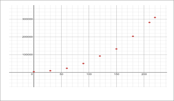
Calculation: Let t = 0 for 1970 then the above table would be written as.
| Year ( t) | Growth ( P) |
| 0 | 3929 |
| 30 | 9638 |
| 60 | 23,192 |
| 90 | 50189 |
| 120 | 92,228 |
| 150 | 132,165 |
| 180 | 203,302 |
| 210 | 281,422 |
| 220 | 309,447 |
Scatter plot of the table data shown below.
c.
To predict: the U.S. population in the 2050.
c.
Answer to Problem 41RE
Explanation of Solution
Given information:
Calculation:
2050 is 260 years after 1970, so t = 260 plug that into the regression equation to find the U.S. population in the 2050.
d.
To find: in what year was the U.S. population growing the fastest and what significant behavior does the graph of the regression equation exhibit at that point
d.
Answer to Problem 41RE
About year 2000.
Explanation of Solution
Given information:
Calculation:
Scatter plot of the table data shown below.

From the graph, the population is increasing the fastest around t =210 .or the year 2000.
The slope of the tangent line at that point is greatest there, in other words, the change in population over the change in time is largest.
The concavity also changes at that point, so it is a point of inflection.
e.
To find: what does the regression equation indicate about the population of Pennsylvania in the long run.
e.
Answer to Problem 41RE
In the long term, the equation says the population will stabilize at around
Explanation of Solution
Given information:
Calculation:
So, in the long term, the equation says the population will stabilize at around
Chapter 5 Solutions
Calculus: Graphical, Numerical, Algebraic
Additional Math Textbook Solutions
Calculus: Early Transcendentals (2nd Edition)
Basic Business Statistics, Student Value Edition
Elementary Statistics (13th Edition)
Introductory Statistics
Intro Stats, Books a la Carte Edition (5th Edition)


- The spread of an infectious disease is often modeled using the following autonomous differential equation: dI - - BI(N − I) − MI, dt where I is the number of infected people, N is the total size of the population being modeled, ẞ is a constant determining the rate of transmission, and μ is the rate at which people recover from infection. Close a) (5 points) Suppose ẞ = 0.01, N = 1000, and µ = 2. Find all equilibria. b) (5 points) For the equilbria in part a), determine whether each is stable or unstable. c) (3 points) Suppose ƒ(I) = d. Draw a phase plot of f against I. (You can use Wolfram Alpha or Desmos to plot the function, or draw the dt function by hand.) Identify the equilibria as stable or unstable in the graph. d) (2 points) Explain the biological meaning of these equilibria being stable or unstable.arrow_forwardFind the indefinite integral. Check Answer: 7x 4 + 1x dxarrow_forwardshow sketcharrow_forward
- Find the indefinite integral. Check Answer: 7x 4 + 1x dxarrow_forwardQuestion 1: Evaluate the following indefinite integrals. a) (5 points) sin(2x) 1 + cos² (x) dx b) (5 points) t(2t+5)³ dt c) (5 points) √ (In(v²)+1) 4 -dv ขarrow_forwardFind the indefinite integral. Check Answer: In(5x) dx xarrow_forward
- Find the indefinite integral. Check Answer: 7x 4 + 1x dxarrow_forwardHere is a region R in Quadrant I. y 2.0 T 1.5 1.0 0.5 0.0 + 55 0.0 0.5 1.0 1.5 2.0 X It is bounded by y = x¹/3, y = 1, and x = 0. We want to evaluate this double integral. ONLY ONE order of integration will work. Good luck! The dA =???arrow_forward43–46. Directions of change Consider the following functions f and points P. Sketch the xy-plane showing P and the level curve through P. Indicate (as in Figure 15.52) the directions of maximum increase, maximum decrease, and no change for f. ■ 45. f(x, y) = x² + xy + y² + 7; P(−3, 3)arrow_forward
 Calculus: Early TranscendentalsCalculusISBN:9781285741550Author:James StewartPublisher:Cengage Learning
 Thomas' Calculus (14th Edition)CalculusISBN:9780134438986Author:Joel R. Hass, Christopher E. Heil, Maurice D. WeirPublisher:PEARSON
 Calculus: Early Transcendentals (3rd Edition)CalculusISBN:9780134763644Author:William L. Briggs, Lyle Cochran, Bernard Gillett, Eric SchulzPublisher:PEARSON
 Calculus: Early TranscendentalsCalculusISBN:9781319050740Author:Jon Rogawski, Colin Adams, Robert FranzosaPublisher:W. H. Freeman
 Calculus: Early Transcendental FunctionsCalculusISBN:9781337552516Author:Ron Larson, Bruce H. EdwardsPublisher:Cengage Learning