Concept explainers
Videos
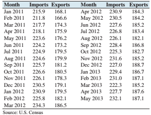
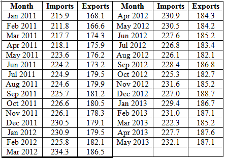
Imports and exports: The following table presents the U.S. imports and exports (in billions of dollars) for each of 29 months.
- Compute the least-squares regression line for predicting exports (y) from imports (x).
- Compute the coefficient of determination.
- The months with the two lowest exports are January and February 2011 Remove these points and compute the least-squares regression line. Is the result noticeably different?
- Compute the coefficient of determination for the data set with January and February 2011 removed.
- Two economists decide to study the relationship between imports and exports. One uses data from January 2011 through May 2013 and the other used data from March 2011 through May 2013. For which data set will the proportion of variance explained by the least-squares regression line be greater?
(a)
>The least squares regression line for the given data set.
Answer to Problem 26E
Explanation of Solution
Given information:
The following table presents the U.S. imports and exports (in billions of dollars) for each of
months:
Concepts Used:
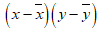
The equation for least-square regression line:
Where
The correlation coefficient of a data is given by:
Where,
The standard deviations are given by:
Calculation:
The mean of
The mean of
The data can be represented in tabular form as:
| x | y |  |
 |
 |
 |
 |
| 215.9 | 168.1 | -10.21724 | 104.39202 | -13.18276 | 173.78512 | 134.69143 |
| 211.8 | 166.6 | -14.31724 | 204.98340 | -14.68276 | 215.58340 | 210.21660 |
| 217.7 | 174.3 | -8.41724 | 70.84995 | -6.98276 | 48.75892 | 58.77556 |
| 218.1 | 175.9 | -8.01724 | 64.27616 | -5.38276 | 28.97409 | 43.15488 |
| 223.6 | 176.2 | -2.51724 | 6.33650 | -5.08276 | 25.83444 | 12.79453 |
| 224.2 | 173.2 | -1.91724 | 3.67581 | -8.08276 | 65.33099 | 15.49660 |
| 224.9 | 179.5 | -1.21724 | 1.48168 | -1.78276 | 3.17823 | 2.17005 |
| 224.6 | 179.9 | -1.51724 | 2.30202 | -1.38276 | 1.91202 | 2.09798 |
| 225.7 | 181.2 | -0.41724 | 0.17409 | -0.08276 | 0.00685 | 0.03453 |
| 226.6 | 180.5 | 0.48276 | 0.23306 | -0.78276 | 0.61271 | -0.37788 |
| 226.1 | 178.3 | -0.01724 | 0.00030 | -2.98276 | 8.89685 | 0.05143 |
| 230.5 | 179.1 | 4.38276 | 19.20857 | -2.18276 | 4.76444 | -9.56650 |
| 230.9 | 179.5 | 4.78276 | 22.87478 | -1.78276 | 3.17823 | -8.52650 |
| 225.8 | 182.1 | -0.31724 | 0.10064 | 0.81724 | 0.66788 | -0.25926 |
| 234.3 | 186.5 | 8.18276 | 66.95754 | 5.21724 | 27.21961 | 42.69143 |
| 230.9 | 184.3 | 4.78276 | 22.87478 | 3.01724 | 9.10375 | 14.43074 |
| 230.5 | 184.2 | 4.38276 | 19.20857 | 2.91724 | 8.51030 | 12.78556 |
| 227.6 | 185.2 | 1.48276 | 2.19857 | 3.91724 | 15.34478 | 5.80832 |
| 226.8 | 183.4 | 0.68276 | 0.46616 | 2.11724 | 4.48271 | 1.44556 |
| 226.1 | 182.1 | -0.01724 | 0.00030 | 0.81724 | 0.66788 | -0.01409 |
| 228.4 | 186.8 | 2.28276 | 5.21099 | 5.51724 | 30.43995 | 12.59453 |
| 225.3 | 182.7 | -0.81724 | 0.66788 | 1.41724 | 2.00857 | -1.15823 |
| 231.6 | 185.2 | 5.48276 | 30.06064 | 3.91724 | 15.34478 | 21.47729 |
| 227.0 | 188.7 | 0.88276 | 0.77926 | 7.41724 | 55.01547 | 6.54763 |
| 229.4 | 186.7 | 3.28276 | 10.77650 | 5.41724 | 29.34650 | 17.78350 |
| 231.0 | 187.1 | 4.88276 | 23.84133 | 5.81724 | 33.84030 | 28.40419 |
| 222.3 | 185.2 | -3.81724 | 14.57133 | 3.91724 | 15.34478 | -14.95306 |
| 227.7 | 187.6 | 1.58276 | 2.50512 | 6.31724 | 39.90754 | 9.99867 |
| 232.1 | 187.1 | 5.98276 | 35.79340 | 5.81724 | 33.84030 | 34.80315 |
|
|
|
|
|
|
Hence, the standard deviation is given by:
And,
Consider,
Putting the values in the formula,
Putting the values to obtain b1,
Putting the values to obtain b0,
Hence, the least-square regression line is given by:
Therefore, the least squares regression line for the given data set is
(b)
>The coefficient of determination.
Answer to Problem 26E
Explanation of Solution
Given information:
Same as part
Calculation:
From part
The coefficient of determination is given by:

Where
Putting the values to obtain Coefficient of Determination,
Therefore, the Coefficient of Determination is
(c)
>The least squares regression line for the given data set by excluding the outlier points and to check if the result is noticeably different.
Answer to Problem 26E
The result is noticeably different.
Explanation of Solution
Given information:
Same as part
The months with two lowest exports are January and February
Concepts used:
The equation for least-square regression line:
Where
The correlation coefficient of a data is given by:
Where,
The standard deviations are given by:
Calculation:
The months with two lowest exports are January and February
Excluding the outlier,
The mean of
The mean of
The data can be represented in tabular form as:
| x | y |  |
 |
 |
 |
 |
| 217.7 | 174.3 | -8.41724 | 70.84995 | -6.98276 | 48.75892 | 58.77556 |
| 218.1 | 175.9 | -8.01724 | 64.27616 | -5.38276 | 28.97409 | 43.15488 |
| 223.6 | 176.2 | -2.51724 | 6.33650 | -5.08276 | 25.83444 | 12.79453 |
| 224.2 | 173.2 | -1.91724 | 3.67581 | -8.08276 | 65.33099 | 15.49660 |
| 224.9 | 179.5 | -1.21724 | 1.48168 | -1.78276 | 3.17823 | 2.17005 |
| 224.6 | 179.9 | -1.51724 | 2.30202 | -1.38276 | 1.91202 | 2.09798 |
| 225.7 | 181.2 | -0.41724 | 0.17409 | -0.08276 | 0.00685 | 0.03453 |
| 226.6 | 180.5 | 0.48276 | 0.23306 | -0.78276 | 0.61271 | -0.37788 |
| 226.1 | 178.3 | -0.01724 | 0.00030 | -2.98276 | 8.89685 | 0.05143 |
| 230.5 | 179.1 | 4.38276 | 19.20857 | -2.18276 | 4.76444 | -9.56650 |
| 230.9 | 179.5 | 4.78276 | 22.87478 | -1.78276 | 3.17823 | -8.52650 |
| 225.8 | 182.1 | -0.31724 | 0.10064 | 0.81724 | 0.66788 | -0.25926 |
| 234.3 | 186.5 | 8.18276 | 66.95754 | 5.21724 | 27.21961 | 42.69143 |
| 230.9 | 184.3 | 4.78276 | 22.87478 | 3.01724 | 9.10375 | 14.43074 |
| 230.5 | 184.2 | 4.38276 | 19.20857 | 2.91724 | 8.51030 | 12.78556 |
| 227.6 | 185.2 | 1.48276 | 2.19857 | 3.91724 | 15.34478 | 5.80832 |
| 226.8 | 183.4 | 0.68276 | 0.46616 | 2.11724 | 4.48271 | 1.44556 |
| 226.1 | 182.1 | -0.01724 | 0.00030 | 0.81724 | 0.66788 | -0.01409 |
| 228.4 | 186.8 | 2.28276 | 5.21099 | 5.51724 | 30.43995 | 12.59453 |
| 225.3 | 182.7 | -0.81724 | 0.66788 | 1.41724 | 2.00857 | -1.15823 |
| 231.6 | 185.2 | 5.48276 | 30.06064 | 3.91724 | 15.34478 | 21.47729 |
| 227.0 | 188.7 | 0.88276 | 0.77926 | 7.41724 | 55.01547 | 6.54763 |
| 229.4 | 186.7 | 3.28276 | 10.77650 | 5.41724 | 29.34650 | 17.78350 |
| 231.0 | 187.1 | 4.88276 | 23.84133 | 5.81724 | 33.84030 | 28.40419 |
| 222.3 | 185.2 | -3.81724 | 14.57133 | 3.91724 | 15.34478 | -14.95306 |
| 227.7 | 187.6 | 1.58276 | 2.50512 | 6.31724 | 39.90754 | 9.99867 |
| 232.1 | 187.1 | 5.98276 | 35.79340 | 5.81724 | 33.84030 | 34.80315 |
|
|
|
|
|
|
Hence, the standard deviation is given by:
And,
Consider, 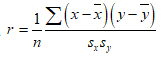
Putting the values in the formula,
Putting the values to obtain
Putting the values to obtain
Hence, the least-square regression line is given by:
Therefore, the least squares regression line for the given data set by removing the outlier is
Hence the result is noticeably different.
(d)
>The coefficient of determination for the data set with the outlier removed.
Answer to Problem 26E
Explanation of Solution
Given information:
Same as part
The months with two lowest exports are January and February
Calculation:
From part
The coefficient of determination is given by:
Where
Plugging the values to obtain Coefficient of Determination,
Therefore, the Coefficient of Determination is
(e)
>To calculate:
To check for which data set will the proportion of variance explained by the least-squares regression line be greater.
Answer to Problem 26E
The proportion of variance explained by the least-squares regression line is greater for the data from January
Explanation of Solution
Given information:
Same as part
Two economists decide to study the relationship between imports and exports. One uses data from January
Calculation:
From previous parts of this exercise,
The Coefficient of Determination is
The Coefficient of Determination without the outliers is
Here the coefficient of determination decreased without the outliers.
Hence, the proportion of variance explained is less without the outlier.
Therefore, the proportion of variance explained by the least-squares regression line is greater for the data from January
Want to see more full solutions like this?
Chapter 4 Solutions
Elementary Statistics (Text Only)


- The following ordered data list shows the data speeds for cell phones used by a telephone company at an airport: A. Calculate the Measures of Central Tendency from the ungrouped data list. B. Group the data in an appropriate frequency table. C. Calculate the Measures of Central Tendency using the table in point B. D. Are there differences in the measurements obtained in A and C? Why (give at least one justified reason)? I leave the answers to A and B to resolve the remaining two. 0.8 1.4 1.8 1.9 3.2 3.6 4.5 4.5 4.6 6.2 6.5 7.7 7.9 9.9 10.2 10.3 10.9 11.1 11.1 11.6 11.8 12.0 13.1 13.5 13.7 14.1 14.2 14.7 15.0 15.1 15.5 15.8 16.0 17.5 18.2 20.2 21.1 21.5 22.2 22.4 23.1 24.5 25.7 28.5 34.6 38.5 43.0 55.6 71.3 77.8 A. Measures of Central Tendency We are to calculate: Mean, Median, Mode The data (already ordered) is: 0.8, 1.4, 1.8, 1.9, 3.2, 3.6, 4.5, 4.5, 4.6, 6.2, 6.5, 7.7, 7.9, 9.9, 10.2, 10.3, 10.9, 11.1, 11.1, 11.6, 11.8, 12.0, 13.1, 13.5, 13.7, 14.1, 14.2, 14.7, 15.0, 15.1, 15.5,…arrow_forwardPEER REPLY 1: Choose a classmate's Main Post. 1. Indicate a range of values for the independent variable (x) that is reasonable based on the data provided. 2. Explain what the predicted range of dependent values should be based on the range of independent values.arrow_forwardIn a company with 80 employees, 60 earn $10.00 per hour and 20 earn $13.00 per hour. Is this average hourly wage considered representative?arrow_forward
- The following is a list of questions answered correctly on an exam. Calculate the Measures of Central Tendency from the ungrouped data list. NUMBER OF QUESTIONS ANSWERED CORRECTLY ON AN APTITUDE EXAM 112 72 69 97 107 73 92 76 86 73 126 128 118 127 124 82 104 132 134 83 92 108 96 100 92 115 76 91 102 81 95 141 81 80 106 84 119 113 98 75 68 98 115 106 95 100 85 94 106 119arrow_forwardThe following ordered data list shows the data speeds for cell phones used by a telephone company at an airport: A. Calculate the Measures of Central Tendency using the table in point B. B. Are there differences in the measurements obtained in A and C? Why (give at least one justified reason)? 0.8 1.4 1.8 1.9 3.2 3.6 4.5 4.5 4.6 6.2 6.5 7.7 7.9 9.9 10.2 10.3 10.9 11.1 11.1 11.6 11.8 12.0 13.1 13.5 13.7 14.1 14.2 14.7 15.0 15.1 15.5 15.8 16.0 17.5 18.2 20.2 21.1 21.5 22.2 22.4 23.1 24.5 25.7 28.5 34.6 38.5 43.0 55.6 71.3 77.8arrow_forwardIn a company with 80 employees, 60 earn $10.00 per hour and 20 earn $13.00 per hour. a) Determine the average hourly wage. b) In part a), is the same answer obtained if the 60 employees have an average wage of $10.00 per hour? Prove your answer.arrow_forward
- The following ordered data list shows the data speeds for cell phones used by a telephone company at an airport: A. Calculate the Measures of Central Tendency from the ungrouped data list. B. Group the data in an appropriate frequency table. 0.8 1.4 1.8 1.9 3.2 3.6 4.5 4.5 4.6 6.2 6.5 7.7 7.9 9.9 10.2 10.3 10.9 11.1 11.1 11.6 11.8 12.0 13.1 13.5 13.7 14.1 14.2 14.7 15.0 15.1 15.5 15.8 16.0 17.5 18.2 20.2 21.1 21.5 22.2 22.4 23.1 24.5 25.7 28.5 34.6 38.5 43.0 55.6 71.3 77.8arrow_forwardBusinessarrow_forwardhttps://www.hawkeslearning.com/Statistics/dbs2/datasets.htmlarrow_forward
- NC Current Students - North Ce X | NC Canvas Login Links - North ( X Final Exam Comprehensive x Cengage Learning x WASTAT - Final Exam - STAT → C webassign.net/web/Student/Assignment-Responses/submit?dep=36055360&tags=autosave#question3659890_9 Part (b) Draw a scatter plot of the ordered pairs. N Life Expectancy Life Expectancy 80 70 600 50 40 30 20 10 Year of 1950 1970 1990 2010 Birth O Life Expectancy Part (c) 800 70 60 50 40 30 20 10 1950 1970 1990 W ALT 林 $ # 4 R J7 Year of 2010 Birth F6 4+ 80 70 60 50 40 30 20 10 Year of 1950 1970 1990 2010 Birth Life Expectancy Ox 800 70 60 50 40 30 20 10 Year of 1950 1970 1990 2010 Birth hp P.B. KA & 7 80 % 5 H A B F10 711 N M K 744 PRT SC ALT CTRLarrow_forwardHarvard University California Institute of Technology Massachusetts Institute of Technology Stanford University Princeton University University of Cambridge University of Oxford University of California, Berkeley Imperial College London Yale University University of California, Los Angeles University of Chicago Johns Hopkins University Cornell University ETH Zurich University of Michigan University of Toronto Columbia University University of Pennsylvania Carnegie Mellon University University of Hong Kong University College London University of Washington Duke University Northwestern University University of Tokyo Georgia Institute of Technology Pohang University of Science and Technology University of California, Santa Barbara University of British Columbia University of North Carolina at Chapel Hill University of California, San Diego University of Illinois at Urbana-Champaign National University of Singapore McGill…arrow_forwardName Harvard University California Institute of Technology Massachusetts Institute of Technology Stanford University Princeton University University of Cambridge University of Oxford University of California, Berkeley Imperial College London Yale University University of California, Los Angeles University of Chicago Johns Hopkins University Cornell University ETH Zurich University of Michigan University of Toronto Columbia University University of Pennsylvania Carnegie Mellon University University of Hong Kong University College London University of Washington Duke University Northwestern University University of Tokyo Georgia Institute of Technology Pohang University of Science and Technology University of California, Santa Barbara University of British Columbia University of North Carolina at Chapel Hill University of California, San Diego University of Illinois at Urbana-Champaign National University of Singapore…arrow_forward
 Linear Algebra: A Modern IntroductionAlgebraISBN:9781285463247Author:David PoolePublisher:Cengage Learning
 Functions and Change: A Modeling Approach to Coll...AlgebraISBN:9781337111348Author:Bruce Crauder, Benny Evans, Alan NoellPublisher:Cengage Learning
 Big Ideas Math A Bridge To Success Algebra 1: Stu...AlgebraISBN:9781680331141Author:HOUGHTON MIFFLIN HARCOURTPublisher:Houghton Mifflin Harcourt
 Glencoe Algebra 1, Student Edition, 9780079039897...AlgebraISBN:9780079039897Author:CarterPublisher:McGraw Hill
 Elementary Linear Algebra (MindTap Course List)AlgebraISBN:9781305658004Author:Ron LarsonPublisher:Cengage Learning