Concept explainers
Videos
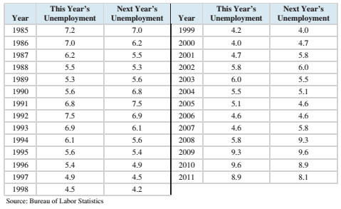
If we are going to use data from this year to predict unemployment next year’s unemployment? A model like this, in which previous values of a variable are used to predict future values of the same variables. Is called an autoregressive model. The following table presents the needed to fit this model.
Compute the least-square line for predicting next year’s unemployment from this year’s unemployment.
To calculate:
To compute the least squares regression line for predicting next year’s unemployment from this year’s unemployment.
Answer to Problem 10CS
Explanation of Solution
Given information:
A model in which previous values of a variable are used to predict future values of the same variable is called an autoregressive model. The following table presents the data needed to fit this model.
| Year | This Year’sUnemployment | Next Year’sUnemployment |
| 1985 | 7.2 | 7.0 |
| 1986 | 7.0 | 6.2 |
| 1987 | 6.2 | 5.5 |
| 1988 | 5.5 | 5.3 |
| 1989 | 5.3 | 5.6 |
| 1990 | 5.6 | 6.8 |
| 1991 | 6.8 | 7.5 |
| 1992 | 7.5 | 6.9 |
| 1993 | 6.9 | 6.1 |
| 1994 | 6.1 | 5.6 |
| 1995 | 5.6 | 5.4 |
| 1996 | 5.4 | 4.9 |
| 1997 | 4.9 | 4.5 |
| 1998 | 4.5 | 4.2 |
| 1999 | 4.2 | 4.0 |
| 2000 | 4.0 | 4.7 |
| 2001 | 4.7 | 5.8 |
| 2002 | 5.8 | 6.0 |
| 2003 | 6.0 | 5.5 |
| 2004 | 5.5 | 5.1 |
| 2005 | 5.1 | 4.6 |
| 2006 | 4.6 | 4.6 |
| 2007 | 4.6 | 5.8 |
| 2008 | 5.8 | 9.3 |
| 2009 | 9.3 | 9.6 |
| 2010 | 9.6 | 8.9 |
| 2011 | 8.9 | 8.1 |
Formula Used:
The equation for least-square regression line:
Where
The correlation coefficient of a data is given by:
Where,
The standard deviations are given by:
The mean of x is given by:
The mean of y is given by:
Calculation:
The mean of x is given by:
The mean of y is given by:
The data can be represented in tabular form as:
| x | y |  |
 |
 |
 |
| 7.2 | 7.0 | 1.17778 | 1.38716 | 0.94444 | 0.89198 |
| 7.0 | 6.2 | 4.12963 | 17.05384 | 0.14444 | 0.02086 |
| 6.2 | 5.5 | 3.32963 | 11.08643 | -0.55556 | 0.30864 |
| 5.5 | 5.3 | 2.62963 | 6.91495 | -0.75556 | 0.57086 |
| 5.3 | 5.6 | 2.42963 | 5.90310 | -0.45556 | 0.20753 |
| 5.6 | 6.8 | 2.72963 | 7.45088 | 0.74444 | 0.55420 |
| 6.8 | 7.5 | 3.92963 | 15.44199 | 1.44444 | 2.08642 |
| 7.5 | 6.9 | 4.62963 | 21.43347 | 0.84444 | 0.71309 |
| 6.9 | 6.1 | 4.02963 | 16.23791 | 0.04444 | 0.00198 |
| 6.1 | 5.6 | 3.22963 | 10.43051 | -0.45556 | 0.20753 |
| 5.6 | 5.4 | 2.72963 | 7.45088 | -0.65556 | 0.42975 |
| 5.4 | 4.9 | 2.52963 | 6.39903 | -1.15556 | 1.33531 |
| 4.9 | 4.5 | 2.02963 | 4.11940 | -1.55556 | 2.41975 |
| 4.5 | 4.2 | 1.62963 | 2.65569 | -1.85556 | 3.44309 |
| 4.2 | 4.0 | 1.32963 | 1.76791 | -2.05556 | 4.22531 |
| 4.0 | 4.7 | 1.12963 | 1.27606 | -1.35556 | 1.83753 |
| 4.7 | 5.8 | 1.82963 | 3.34754 | -0.25556 | 0.06531 |
| 5.8 | 6.0 | 2.92963 | 8.58273 | -0.05556 | 0.00309 |
| 6.0 | 5.5 | 3.12963 | 9.79458 | -0.55556 | 0.30864 |
| 5.5 | 5.1 | 2.62963 | 6.91495 | -0.95556 | 0.91309 |
| 5.1 | 4.6 | 2.22963 | 4.97125 | -1.45556 | 2.11864 |
| 4.6 | 4.6 | 1.72963 | 2.99162 | -1.45556 | 2.11864 |
| 4.6 | 5.8 | 1.72963 | 2.99162 | -0.25556 | 0.06531 |
| 5.8 | 9.3 | 2.92963 | 8.58273 | 3.24444 | 10.52642 |
| 9.3 | 9.6 | 6.42963 | 41.34014 | 3.54444 | 12.56309 |
| 9.6 | 8.9 | 6.72963 | 45.28791 | 2.84444 | 8.09086 |
| 8.9 | 8.1 | 6.02963 | 36.35643 | 2.04444 | 4.17975 |
| |
|
|
|
Hence, the standard deviation is given by:
And,
Consider,
Hence, the table for calculating coefficient of correlation is given by:
| x | y |  |
 |
 |
| 7.2 | 7.0 | 1.17778 | 0.94444 | 1.11235 |
| 7.0 | 6.2 | 4.12963 | 0.14444 | 0.59650 |
| 6.2 | 5.5 | 3.32963 | -0.55556 | -1.84979 |
| 5.5 | 5.3 | 2.62963 | -0.75556 | -1.98683 |
| 5.3 | 5.6 | 2.42963 | -0.45556 | -1.10683 |
| 5.6 | 6.8 | 2.72963 | 0.74444 | 2.03206 |
| 6.8 | 7.5 | 3.92963 | 1.44444 | 5.67613 |
| 7.5 | 6.9 | 4.62963 | 0.84444 | 3.90947 |
| 6.9 | 6.1 | 4.02963 | 0.04444 | 0.17909 |
| 6.1 | 5.6 | 3.22963 | -0.45556 | -1.47128 |
| 5.6 | 5.4 | 2.72963 | -0.65556 | -1.78942 |
| 5.4 | 4.9 | 2.52963 | -1.15556 | -2.92313 |
| 4.9 | 4.5 | 2.02963 | -1.55556 | -3.15720 |
| 4.5 | 4.2 | 1.62963 | -1.85556 | -3.02387 |
| 4.2 | 4.0 | 1.32963 | -2.05556 | -2.73313 |
| 4.0 | 4.7 | 1.12963 | -1.35556 | -1.53128 |
| 4.7 | 5.8 | 1.82963 | -0.25556 | -0.46757 |
| 5.8 | 6.0 | 2.92963 | -0.05556 | -0.16276 |
| 6.0 | 5.5 | 3.12963 | -0.55556 | -1.73868 |
| 5.5 | 5.1 | 2.62963 | -0.95556 | -2.51276 |
| 5.1 | 4.6 | 2.22963 | -1.45556 | -3.24535 |
| 4.6 | 4.6 | 1.72963 | -1.45556 | -2.51757 |
| 4.6 | 5.8 | 1.72963 | -0.25556 | -0.44202 |
| 5.8 | 9.3 | 2.92963 | 3.24444 | 9.50502 |
| 9.3 | 9.6 | 6.42963 | 3.54444 | 22.78947 |
| 9.6 | 8.9 | 6.72963 | 2.84444 | 19.14206 |
| 8.9 | 8.1 | 6.02963 | 2.04444 | 12.32724 |
| |
|
|
Plugging the values in the formula,
Plugging the values to obtain b1,
Plugging the values to obtain b0,
Hence, the least-square regression line is given by:
Therefore, the least squares regression line for the given data set is
Want to see more full solutions like this?
Chapter 4 Solutions
Elementary Statistics (Text Only)


- A company found that the daily sales revenue of its flagship product follows a normal distribution with a mean of $4500 and a standard deviation of $450. The company defines a "high-sales day" that is, any day with sales exceeding $4800. please provide a step by step on how to get the answers in excel Q: What percentage of days can the company expect to have "high-sales days" or sales greater than $4800? Q: What is the sales revenue threshold for the bottom 10% of days? (please note that 10% refers to the probability/area under bell curve towards the lower tail of bell curve) Provide answers in the yellow cellsarrow_forwardFind the critical value for a left-tailed test using the F distribution with a 0.025, degrees of freedom in the numerator=12, and degrees of freedom in the denominator = 50. A portion of the table of critical values of the F-distribution is provided. Click the icon to view the partial table of critical values of the F-distribution. What is the critical value? (Round to two decimal places as needed.)arrow_forwardA retail store manager claims that the average daily sales of the store are $1,500. You aim to test whether the actual average daily sales differ significantly from this claimed value. You can provide your answer by inserting a text box and the answer must include: Null hypothesis, Alternative hypothesis, Show answer (output table/summary table), and Conclusion based on the P value. Showing the calculation is a must. If calculation is missing,so please provide a step by step on the answers Numerical answers in the yellow cellsarrow_forward
 Glencoe Algebra 1, Student Edition, 9780079039897...AlgebraISBN:9780079039897Author:CarterPublisher:McGraw Hill
 Elementary Linear Algebra (MindTap Course List)AlgebraISBN:9781305658004Author:Ron LarsonPublisher:Cengage Learning
 College Algebra (MindTap Course List)AlgebraISBN:9781305652231Author:R. David Gustafson, Jeff HughesPublisher:Cengage Learning
 Big Ideas Math A Bridge To Success Algebra 1: Stu...AlgebraISBN:9781680331141Author:HOUGHTON MIFFLIN HARCOURTPublisher:Houghton Mifflin Harcourt