Chapter 4, Problem 2CS

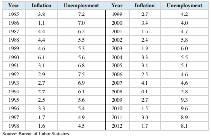
The following table, Reproduce from chapter introduction. Presents the inflation rate and unemployment rate, both in percent, for the years 1985-2012

We will investigate some methods for predicting unemployment first. We will try to predict the unemployment rate from the inflation rate.

Compute the least-squares line for predicting unemployment from inflation.

To determine

To calculate: To compute the least squares regression line for the given data set.

Answer to Problem 2CS

  $y=-0.199x+6.6594$

Explanation of Solution

Given information:

The following table presents the inflation rate and unemployment rate, both in percent, for the years 1985-2012.

Year	Inflation	Unemployment
1985	3.8	7.2
1986	1.1	7.0
1987	4.4	6.2
1988	4.4	5.5
1989	4.6	5.3
1990	6.1	5.6
1991	3.1	6.8
1992	2.9	7.5
1993	2.7	6.9
1994	2.7	6.1
1995	2.5	5.6
1996	3.3	5.4
1997	1.7	4.9
1998	1.6	4.5
1999	2.7	4.2
2000	3.4	4.0
2001	1.6	4.7
2002	2.4	5.8
2003	1.9	6.0
2004	3.3	5.5
2005	3.4	5.1
2006	2.5	4.6
2007	4.1	4.6
2008	0.1	5.8
2009	2.7	9.3
2010	1.5	9.6
2011	3.0	8.9
2012	1.7	8.1

Formula Used:

The equation for least-square regression line:

  $y=b_0+b_{1}x$

Where $b_1=r\frac{s_y}{s_x}$ is the slope and $b_0=\overline{y}-b_1\overline{x}$ is the y -intercept.

The correlation coefficient of a data is given by:

  $r=\frac{1}{n}\frac{{\displaystyle \sum \left(x-\overline{x}\right)\left(y-\overline{y}\right)}}{s_x{s}_y}$

Where,

  $\overline{x},\overline{y}$ represent the mean of x and y respectively. $s_x,s_y$ represent the standard deviations of x and y . n represents the number of terms.

The standard deviations are given by:

  $s_x=\sqrt{\frac{{\displaystyle \sum {\left(x-\overline{x}\right)}^2}}{n}},s_y=\sqrt{\frac{{\displaystyle \sum {\left(y-\overline{y}\right)}^2}}{n}}$

The mean of x is given by:

  $\overline{x}=\frac{{\displaystyle \sum x}}{n}$

The mean of y is given by:

  $\overline{y}=\frac{{\displaystyle \sum y}}{n}$

Calculation:

The mean of x is given by:

  $\begin{array}{l}\overline{x}=\frac{{\displaystyle \sum x}}{n}=\frac{\begin{array}{l}3.8+1.1+4.4+4.4+4.6+6.1+3.1+2.9+2.7+2.7+2.5+3.3+1.7+1.6+\\ 2.7+3.4+1.6+2.4+1.9+3.3+3.4+2.5+4.1+0.1+2.7+1.5+3.0+1.7\end{array}}{28}\\ \overline{x}=\frac{{\displaystyle \sum x}}{n}=\frac{79.20}{28}=2.82857\end{array}$

The mean of y is given by:

  $\begin{array}{l}\overline{y}=\frac{{\displaystyle \sum y}}{n}=\frac{\begin{array}{l}7.2+7.0+6.2+5.5+5.3+5.6+6.8+7.5+6.9+6.1+5.6+5.4+4.9+4.5+\\ 4.2+4.0+4.7+5.8+6.0+5.5+5.1+4.6+4.6+5.8+9.3+9.6+8.9+8.1\end{array}}{28}\\ \overline{y}=\frac{{\displaystyle \sum y}}{n}=\frac{170.7}{28}=6.09643\end{array}$

The data can be represented in tabular form as:

x	y
3.8	7.2	0.97143	0.94367	1.10357	1.21787
1.1	7.0	-1.72857	2.98796	0.90357	0.81644
4.4	6.2	1.57143	2.46939	0.10357	0.01073
4.4	5.5	1.57143	2.46939	-0.59643	0.35573
4.6	5.3	1.77143	3.13796	-0.79643	0.63430
6.1	5.6	3.27143	10.70224	-0.49643	0.24644
3.1	6.8	0.27143	0.07367	0.70357	0.49501
2.9	7.5	0.07143	0.00510	1.40357	1.97001
2.7	6.9	-0.12857	0.01653	0.80357	0.64573
2.7	6.1	-0.12857	0.01653	0.00357	0.00001
2.5	5.6	-0.32857	0.10796	-0.49643	0.24644
3.3	5.4	0.47143	0.22224	-0.69643	0.48501
1.7	4.9	-1.12857	1.27367	-1.19643	1.43144
1.6	4.5	-1.22857	1.50939	-1.59643	2.54858
2.7	4.2	-0.12857	0.01653	-1.89643	3.59644
3.4	4.0	0.57143	0.32653	-2.09643	4.39501
1.6	4.7	-1.22857	1.50939	-1.39643	1.95001
2.4	5.8	-0.42857	0.18367	-0.29643	0.08787
1.9	6.0	-0.92857	0.86224	-0.09643	0.00930
3.3	5.5	0.47143	0.22224	-0.59643	0.35573
3.4	5.1	0.57143	0.32653	-0.99643	0.99287
2.5	4.6	-0.32857	0.10796	-1.49643	2.23930
4.1	4.6	1.27143	1.61653	-1.49643	2.23930
0.1	5.8	-2.72857	7.44510	-0.29643	0.08787
2.7	9.3	-0.12857	0.01653	3.20357	10.26287
1.5	9.6	-1.32857	1.76510	3.50357	12.27501
3.0	8.9	0.17143	0.02939	2.80357	7.86001
1.7	8.1	-1.12857	1.27367	2.00357	4.01430
$\overline{x}=2.82857$	$\overline{y}=6.09643$		$\begin{array}{l}{\displaystyle \sum {\left(x-\overline{x}\right)}^2}=\\ 41.63714\end{array}$		$\begin{array}{l}{\displaystyle \sum {\left(y-\overline{y}\right)}^2}=\\ 61.46964\end{array}$

Hence, the standard deviation is given by:

  $\begin{array}{l}{s}_x=\sqrt{\frac{{\displaystyle \sum {\left(x-\overline{x}\right)}^2}}{n}}\\ s_x=\sqrt{\frac{41.63714}{28}}\\ s_x=\sqrt{1.48704}\end{array}$

And,

  $\begin{array}{l}{s}_y=\sqrt{\frac{{\displaystyle \sum {\left(y-\overline{y}\right)}^2}}{n}}\\ s_y=\sqrt{\frac{61.46964}{28}}\\ s_y=\sqrt{2.19534}\end{array}$

Consider, $r=\frac{1}{n}\frac{{\displaystyle \sum \left(x-\overline{x}\right)\left(y-\overline{y}\right)}}{s_x{s}_y}$

Hence, the table for calculating coefficient of correlation is given by:

x	y
3.8	7.2	0.97143	1.10357	1.07204
1.1	7.0	-1.72857	0.90357	-1.56189
4.4	6.2	1.57143	0.10357	0.16276
4.4	5.5	1.57143	-0.59643	-0.93724
4.6	5.3	1.77143	-0.79643	-1.41082
6.1	5.6	3.27143	-0.49643	-1.62403
3.1	6.8	0.27143	0.70357	0.19097
2.9	7.5	0.07143	1.40357	0.10026
2.7	6.9	-0.12857	0.80357	-0.10332
2.7	6.1	-0.12857	0.00357	-0.00046
2.5	5.6	-0.32857	-0.49643	0.16311
3.3	5.4	0.47143	-0.69643	-0.32832
1.7	4.9	-1.12857	-1.19643	1.35026
1.6	4.5	-1.22857	-1.59643	1.96133
2.7	4.2	-0.12857	-1.89643	0.24383
3.4	4.0	0.57143	-2.09643	-1.19796
1.6	4.7	-1.22857	-1.39643	1.71561
2.4	5.8	-0.42857	-0.29643	0.12704
1.9	6.0	-0.92857	-0.09643	0.08954
3.3	5.5	0.47143	-0.59643	-0.28117
3.4	5.1	0.57143	-0.99643	-0.56939
2.5	4.6	-0.32857	-1.49643	0.49168
4.1	4.6	1.27143	-1.49643	-1.90260
0.1	5.8	-2.72857	-0.29643	0.80883
2.7	9.3	-0.12857	3.20357	-0.41189
1.5	9.6	-1.32857	3.50357	-4.65474
3.0	8.9	0.17143	2.80357	0.48061
1.7	8.1	-1.12857	2.00357	-2.26117
$\overline{x}=2.82857$	$\overline{y}=6.09643$			$\begin{array}{l}{\displaystyle \sum \left(x-\overline{x}\right)\left(y-\overline{y}\right)}=\\ -8.28714\end{array}$

Plugging the values in the formula,

  $\begin{array}{l}r=\frac{1}{n}\frac{{\displaystyle \sum \left(x-\overline{x}\right)\left(y-\overline{y}\right)}}{s_x{s}_y}\\ r=\frac{1}{28}\cdot \frac{-8.28714}{\left(\sqrt{1.48704}\right)\left(\sqrt{2.19534}\right)}\\ r=-0.16381\end{array}$

Plugging the values to obtain b₁ ,

  $\begin{array}{l}{b}_1=r\frac{s_y}{s_x}\\ b_1=\frac{1}{28}\cdot \frac{-8.28714}{\left(\sqrt{1.48704}\right)\left(\sqrt{2.19534}\right)}\frac{\left(\sqrt{2.19534}\right)}{\left(\sqrt{1.48704}\right)}\\ b_1=-0.1990\end{array}$

Plugging the values to obtain b₀ ,

  $\begin{array}{l}{b}_0=\overline{y}-b_1\overline{x}\\ b_0=\left(6.09643\right)-\left(-0.1990\right)\left(2.82857\right)\\ b_0=6.6594\end{array}$

Hence, the least-square regression line is given by:

  $\begin{array}{l}y=b_0+b_{1}x\\ y=\left(6.6594\right)+\left(-0.1990\right)x\\ y=-0.199x+6.6594\end{array}$

Therefore, the least squares regression line for the given data set is $y=-0.199x+6.6594$