Chapter 4, Problem 6CS

The relationship between inflation and unemployment is not very strong. However .if we are interested in predicting unemployment, we would probably want to predict next year’s unemployment from this year’s inflation we can construct equation to do this by matching each year? Inflation with the next year’s unemployment. As shown in the following table.

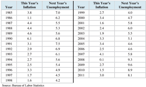
Compute the least-squares line for predicting next year’s unemployment from this year’s inflation

To determine

To calculate:

To compute the least squares regression line for the given data set.

Answer to Problem 6CS

$y=-0.2251x+6.7017$

Explanation of Solution

Given information:

The following table presents the inflation rate and unemployment rate, both in percent, for the years 1985-2012.

Year	Inflation	Unemployment
1985	3.8	7.0
1986	1.1	6.2
1987	4.4	5.5
1988	4.4	5.3
1989	4.6	5.6
1990	6.1	6.8
1991	3.1	7.5
1992	2.9	6.9
1993	2.7	6.1
1994	2.7	5.6
1995	2.5	5.4
1996	3.3	4.9
1997	1.7	4.5
1998	1.6	4.2
1999	2.7	4.0
2000	3.4	4.7
2001	1.6	5.8
2002	2.4	6.0
2003	1.9	5.5
2004	3.3	5.1
2005	3.4	4.6
2006	2.5	4.6
2007	4.1	5.8
2008	0.1	9.3
2009	2.7	9.6
2010	1.5	8.9
2011	3.0	8.1

Formula Used:

The equation for least-square regression line:

$y=b_0+b_{1}x$

Where $b_1=r\frac{s_y}{s_x}$ is the slope and $b_0=\overline{y}-b_1\overline{x}$ is the y -intercept.

The correlation coefficient of a data is given by:

$r=\frac{1}{n}\frac{{\displaystyle \sum \left(x-\overline{x}\right)\left(y-\overline{y}\right)}}{s_x{s}_y}$

Where,

$\overline{x},\overline{y}$ represent the mean of x and y respectively. $s_x,s_y$ represent the standard deviations of x and y. n represents the number of terms.

The standard deviations are given by:

$s_x=\sqrt{\frac{{\displaystyle \sum {\left(x-\overline{x}\right)}^2}}{n}},s_y=\sqrt{\frac{{\displaystyle \sum {\left(y-\overline{y}\right)}^2}}{n}}$

The mean of x is given by:

$\overline{x}=\frac{{\displaystyle \sum x}}{n}$

The mean of y is given by:

$\overline{y}=\frac{{\displaystyle \sum y}}{n}$

Calculation:

The mean of x is given by:

$\begin{array}{l}\overline{x}=\frac{{\displaystyle \sum x}}{n}=\frac{\begin{array}{l}3.8+1.1+4.4+4.4+4.6+6.1+3.1+2.9+2.7+2.7+2.5+3.3+1.7+1.6+\\ 2.7+3.4+1.6+2.4+1.9+3.3+3.4+2.5+4.1+0.1+2.7+1.5+3.0\end{array}}{27}\\ \overline{x}=\frac{{\displaystyle \sum x}}{n}=\frac{77.50}{27}=2.87037\end{array}$

The mean of y is given by:

$\begin{array}{l}\overline{y}=\frac{{\displaystyle \sum y}}{n}=\frac{\begin{array}{l}7.0+6.2+5.5+5.3+5.6+6.8+7.5+6.9+6.1+5.6+5.4+4.9+4.5+\\ 4.2+4.0+4.7+5.8+6.0+5.5+5.1+4.6+4.6+5.8+9.3+9.6+8.9+8.1\end{array}}{27}\\ \overline{y}=\frac{{\displaystyle \sum y}}{n}=\frac{163.5}{27}=6.05556\end{array}$

The data can be represented in tabular form as:

x	y
3.8	7.0	0.92963	0.86421	0.94444	0.89198
1.1	6.2	-1.77037	3.13421	0.14444	0.02086
4.4	5.5	1.52963	2.33977	-0.55556	0.30864
4.4	5.3	1.52963	2.33977	-0.75556	0.57086
4.6	5.6	1.72963	2.99162	-0.45556	0.20753
6.1	6.8	3.22963	10.43051	0.74444	0.55420
3.1	7.5	0.22963	0.05273	1.44444	2.08642
2.9	6.9	0.02963	0.00088	0.84444	0.71309
2.7	6.1	-0.17037	0.02903	0.04444	0.00198
2.7	5.6	-0.17037	0.02903	-0.45556	0.20753
2.5	5.4	-0.37037	0.13717	-0.65556	0.42975
3.3	4.9	0.42963	0.18458	-1.15556	1.33531
1.7	4.5	-1.17037	1.36977	-1.55556	2.41975
1.6	4.2	-1.27037	1.61384	-1.85556	3.44309
2.7	4.0	-0.17037	0.02903	-2.05556	4.22531
3.4	4.7	0.52963	0.28051	-1.35556	1.83753
1.6	5.8	-1.27037	1.61384	-0.25556	0.06531
2.4	6.0	-0.47037	0.22125	-0.05556	0.00309
1.9	5.5	-0.97037	0.94162	-0.55556	0.30864
3.3	5.1	0.42963	0.18458	-0.95556	0.91309
3.4	4.6	0.52963	0.28051	-1.45556	2.11864
2.5	4.6	-0.37037	0.13717	-1.45556	2.11864
4.1	5.8	1.22963	1.51199	-0.25556	0.06531
0.1	9.3	-2.77037	7.67495	3.24444	10.52642
2.7	9.6	-0.17037	0.02903	3.54444	12.56309
1.5	8.9	-1.37037	1.87791	2.84444	8.09086
3.0	8.1	0.12963	0.01680	2.04444	4.17975
$\overline{x}=2.87037$	$\overline{y}=6.05556$		$\begin{array}{l}{\displaystyle \sum {\left(x-\overline{x}\right)}^2}=\\ 40.31630\end{array}$		$\begin{array}{l}{\displaystyle \sum {\left(y-\overline{y}\right)}^2}=\\ 60.20667\end{array}$

Hence, the standard deviation is given by:

$\begin{array}{l}{s}_x=\sqrt{\frac{{\displaystyle \sum {\left(x-\overline{x}\right)}^2}}{n}}\\ s_x=\sqrt{\frac{40.31630}{27}}\\ s_x=\sqrt{1.49320}\end{array}$

And,

$\begin{array}{l}{s}_y=\sqrt{\frac{{\displaystyle \sum {\left(y-\overline{y}\right)}^2}}{n}}\\ s_y=\sqrt{\frac{60.20667}{27}}\\ s_y=\sqrt{2.22988}\end{array}$

Consider, $r=\frac{1}{n}\frac{{\displaystyle \sum \left(x-\overline{x}\right)\left(y-\overline{y}\right)}}{s_x{s}_y}$

Hence, the table for calculating coefficient of correlation is given by:

x	y
3.8	7.0	0.92963	0.94444	0.87798
1.1	6.2	-1.77037	0.14444	-0.25572
4.4	5.5	1.52963	-0.55556	-0.84979
4.4	5.3	1.52963	-0.75556	-1.15572
4.6	5.6	1.72963	-0.45556	-0.78794
6.1	6.8	3.22963	0.74444	2.40428
3.1	7.5	0.22963	1.44444	0.33169
2.9	6.9	0.02963	0.84444	0.02502
2.7	6.1	-0.17037	0.04444	-0.00757
2.7	5.6	-0.17037	-0.45556	0.07761
2.5	5.4	-0.37037	-0.65556	0.24280
3.3	4.9	0.42963	-1.15556	-0.49646
1.7	4.5	-1.17037	-1.55556	1.82058
1.6	4.2	-1.27037	-1.85556	2.35724
2.7	4.0	-0.17037	-2.05556	0.35021
3.4	4.7	0.52963	-1.35556	-0.71794
1.6	5.8	-1.27037	-0.25556	0.32465
2.4	6.0	-0.47037	-0.05556	0.02613
1.9	5.5	-0.97037	-0.55556	0.53909
3.3	5.1	0.42963	-0.95556	-0.41053
3.4	4.6	0.52963	-1.45556	-0.77091
2.5	4.6	-0.37037	-1.45556	0.53909
4.1	5.8	1.22963	-0.25556	-0.31424
0.1	9.3	-2.77037	3.24444	-8.98831
2.7	9.6	-0.17037	3.54444	-0.60387
1.5	8.9	-1.37037	2.84444	-3.89794
3.0	8.1	0.12963	2.04444	0.26502
$\overline{x}=2.87037$	$\overline{y}=6.05556$			$\begin{array}{l}{\displaystyle \sum \left(x-\overline{x}\right)\left(y-\overline{y}\right)}=\\ -9.07556\end{array}$

Plugging the values in the formula,

$\begin{array}{l}r=\frac{1}{n}\frac{{\displaystyle \sum \left(x-\overline{x}\right)\left(y-\overline{y}\right)}}{s_x{s}_y}\\ r=\frac{1}{27}\cdot \frac{-9.07556}{\left(\sqrt{1.49320}\right)\left(\sqrt{2.22988}\right)}\\ r=-0.18421\end{array}$

Plugging the values to obtain b₁,

$\begin{array}{l}{b}_1=r\frac{s_y}{s_x}\\ b_1=\frac{1}{27}\cdot \frac{-9.07556}{\left(\sqrt{1.49320}\right)\left(\sqrt{2.22988}\right)}\frac{\left(\sqrt{2.22988}\right)}{\left(\sqrt{1.49320}\right)}\\ b_1=-0.2251\end{array}$

Plugging the values to obtain b₀,

$\begin{array}{l}{b}_0=\overline{y}-b_1\overline{x}\\ b_0=\left(6.05556\right)-\left(-0.2251\right)\left(2.87037\right)\\ b_0=6.7017\end{array}$

Hence, the least-square regression line is given by:

$\begin{array}{l}y=b_0+b_{1}x\\ y=\left(6.7017\right)+\left(-0.2251\right)x\\ y=-0.2251x+6.7017\end{array}$

Therefore, the least squares regression line for the given data set is $y=-0.2251x+6.7017$