Concept explainers
Videos
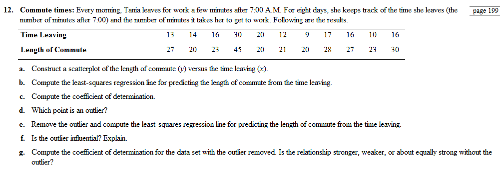
Commute times: Every morning, Tania leaves for work a few minutes after 7:00 A.M. For eight days, she keeps track of the time she leaves (the number of minutes after 7:00) and the number of minutes it takes her to get to work. Following are the results.
- Construct a
scatterplot of the length of commute (y) versus the time leaving (x). - Compute the least-squares regression line for predicting the length of commute from the time leaving.
- Compute the coefficient of determination.
- Which point is an outlier?
- Remove the outlier and compute the least-squares regression line for predicting the length of commute from the time leaving.
- Is the outlier influential? Explain.
- Compute the coefficient of determination for the data set with the outlier removed. Is the relationship stronger. weaker; or about equally strong without the outlier?
a.
To Graph:a scatter plot using the length of commute time
Explanation of Solution
Given information: T leaves her home every day few minutes after
Graph:The scatter plot shows the number of minutes after
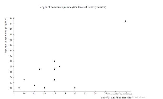
Interpretation:Each of the data in the table contributes an ordered pair of the form (number of minutes after
We use a scatter plot for this example because to understand the relationship between the two variables as ordered pairs it is useful. The points tend to cluster around the straight line. Therefore, we conclude that the variable on the
Now consider the three points
Therefore, we conclude that the variable on the
Because for positive linear relationship the large value of data associates with large values of data in the plot, while for negative linear relationship the large value of data associates with small values of data in the pot. And in this case, it is difficult to say that because the large values of data associate with both small and large and small values of data associate with both small and large at the same time.
Therefore it is good to measure how strong the linear relationship is, to know this we can calculate the correlation coefficient.
b.
To Calculate: the least square regression line
Answer to Problem 12RE
When two variables have a linear relationship, the points on a scatter plot tend to cluster around a straight line called the least square regression line. It is simplified to be
Explanation of Solution
Given information: T leaves her home every day few minutes after
Formulas Used:
Sample mean:
Sample variance:
Correlation Coefficient:
The least-square regression line:
Calculation: Using the below table for calculation.
The sample means and the sample variances can be calculated as shown.
Now, one can use these to calculate the correlation coefficient as shown.
Finally, to calculate the least square regression line as shown, theser can be used.
Where
c.
To Calculate: the coefficient of determination
Answer to Problem 12RE
The coefficient of determination is
Explanation of Solution
Given information: T leaves her home every day few minutes after
Formulas Used:
Sample mean:
Sample variance:
Correlation Coefficient:
Calculation: the correlation coefficient can be calculated as shown by using the formula.
The correlation coefficient
indicates a positive linear association. Here the value of the correlation coefficient close to zero.
Therefore, one can conclude that the positive linear relationship is weak.
Also,
To calculate the coefficient of determination we need to square the correlation coefficient.
Therefore, the coefficient of determination is
d.
To Find: the outlier point
Explanation of Solution
Given information: Tania leaves her home every day few minutes after
Graph: The scatter plot shows the number of minutes after
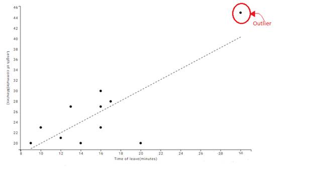
Interpretation: An outlier is a value that considerably larger or considerably smaller than most of the values in a data set. It may be resulting from an error in the process of sampling.
So in the given data set, an outlier point can be detected in the ordered pair
Because it is much larger than the other ordered pairs.
e.
To Calculate: the least square regression line without the outlier point.
Answer to Problem 12RE
The least square regression line without theoutlier point is
Explanation of Solution
Given information: T leaves her home every day few minutes after
Formulas Used:
Sample mean:
Sample variance:
Correlation Coefficient:
The least square regression line:
Calculation: the sample means and the sample variances can be calculated as shown without the outlier point.
Now, one can use these to calculate the correlation coefficient without the outlier as shown.
Finally, one can use these to calculate the least square regression line as shown.
Where
f.
To Show: the outlier is influential
Answer to Problem 12RE
No, the outlier is not that much influential.
Explanation of Solution
Given information: T leaves her home every day few minutes after
The least-square regression line with the outlier is
The least-square regression line without the outlier is
The two least square regression lines are so much close and have no huge difference.
Therefore we can conclude that the outlier is not that much influential. Here, the outlier cannot be a result of an error. It is just random data measured along with the other data in the sampling process.
g.
To Find: the coefficient of determination without the outlier and discuss its strength.
Answer to Problem 12RE
Coefficient of determination is
Explanation of Solution
Given information: T leaves her home every day few minutes after
Formula Used:Sample mean:
Sample variance:
Correlation Coefficient:
Calculation: to calculate the correlation coefficient without the outlier as shown.
The correlation coefficient
indicates a positive linear association. It is
The value is so close to zero .because of the ten to the power is minus thirty-one.
Therefore, one can conclude that the positive linear relationship is very weak without the outlier.
Also,
One can calculate the coefficient of determination by squaring the correlation coefficient.
Therefore, the coefficient of determination is
Want to see more full solutions like this?
Chapter 4 Solutions
Elementary Statistics (Text Only)


- A marketing agency wants to determine whether different advertising platforms generate significantly different levels of customer engagement. The agency measures the average number of daily clicks on ads for three platforms: Social Media, Search Engines, and Email Campaigns. The agency collects data on daily clicks for each platform over a 10-day period and wants to test whether there is a statistically significant difference in the mean number of daily clicks among these platforms. Conduct ANOVA test. You can provide your answer by inserting a text box and the answer must include: also please provide a step by on getting the answers in excel Null hypothesis, Alternative hypothesis, Show answer (output table/summary table), and Conclusion based on the P value.arrow_forwardA company found that the daily sales revenue of its flagship product follows a normal distribution with a mean of $4500 and a standard deviation of $450. The company defines a "high-sales day" that is, any day with sales exceeding $4800. please provide a step by step on how to get the answers Q: What percentage of days can the company expect to have "high-sales days" or sales greater than $4800? Q: What is the sales revenue threshold for the bottom 10% of days? (please note that 10% refers to the probability/area under bell curve towards the lower tail of bell curve) Provide answers in the yellow cellsarrow_forwardBusiness Discussarrow_forward
- The following data represent total ventilation measured in liters of air per minute per square meter of body area for two independent (and randomly chosen) samples. Analyze these data using the appropriate non-parametric hypothesis testarrow_forwardeach column represents before & after measurements on the same individual. Analyze with the appropriate non-parametric hypothesis test for a paired design.arrow_forwardShould you be confident in applying your regression equation to estimate the heart rate of a python at 35°C? Why or why not?arrow_forward
 College AlgebraAlgebraISBN:9781305115545Author:James Stewart, Lothar Redlin, Saleem WatsonPublisher:Cengage Learning
 Elementary Linear Algebra (MindTap Course List)AlgebraISBN:9781305658004Author:Ron LarsonPublisher:Cengage Learning
 Algebra and Trigonometry (MindTap Course List)AlgebraISBN:9781305071742Author:James Stewart, Lothar Redlin, Saleem WatsonPublisher:Cengage Learning
 Functions and Change: A Modeling Approach to Coll...AlgebraISBN:9781337111348Author:Bruce Crauder, Benny Evans, Alan NoellPublisher:Cengage Learning
 Linear Algebra: A Modern IntroductionAlgebraISBN:9781285463247Author:David PoolePublisher:Cengage Learning