
Concept explainers
Videos
To determine: Find the forecast of sales using exponential smoothing with smoothing constant 0.6 and 0.9 and infer the effect of exponential smoothing on forecast. Using MAD, determine the accurate forecast of exponential smoothing with given smoothing constant 0.3, 0.6 and 0.9.
Introduction: A sequence of data points in successive order is known as time series. Time series
Answer to Problem 17P
On Comparing MAD from exponential smoothing with smoothing constant 0.3, 0.6 and 0.9 (refer to equations (1), (2) and (3)), it can be inferred that the MAD of exponential smoothing with smoothing constant is most accurate because of least value of MAD.
Explanation of Solution
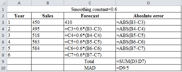
Forecast of sales using exponential smoothing with smoothing constant 0.6:
Given information:
| Year | Sales |
| 1 | 450 |
| 2 | 495 |
| 3 | 518 |
| 4 | 563 |
| 5 | 584 |
Formula to calculate the forecasted demand:
Where,
| Smoothing constant=0.6 | |||
| Year | Sales | Forecast | Absolute error |
| 1 | 450 | 410 | 40 |
| 2 | 495 | 434 | 61 |
| 3 | 518 | 470.6 | 47.4 |
| 4 | 563 | 499.04 | 63.96 |
| 5 | 584 | 537.416 | 46.584 |
| 6 | 565.3664 | ||
| Total | 258.944 | ||
| MAD | 51.7888 | ||
Excel worksheet:
Calculation of the forecast for year 2:
To calculate the forecast for year 2, substitute the value of forecast of year 1, smoothing constant and the difference of actual and forecasted demand in the above formula. The result of the forecast for year 2 is 434.
Calculation of the forecast for year 3:
To calculate the forecast for year 3, substitute the value of forecast of year 2, smoothing constant and the difference of actual and forecasted demand in the above formula. The result of the forecast for year 3 is 470.6.
Calculation of the forecast for year 4:
To calculate the forecast for year 4, substitute the value of forecast of year 3, smoothing constant and the difference of actual and forecasted demand in the above formula. The result of the forecast for year 4 is 499.04.
Calculation of the forecast for year 5:
To calculate the forecast for year 5, substitute the value of forecast of year 4, smoothing constant and the difference of actual and forecasted demand in the above formula. The result of the forecast for year 5 is 537.416.
Calculation of the forecast for year 6:
To calculate the forecast for year 5, substitute the value of forecast of year 5, smoothing constant and the difference of actual and forecasted demand in the above formula. The result of the forecast for year 6 is 565.36.
Calculation of MAD using exponential smoothing with smoothing constant α=0.6:
Formula to calculate the Mean Absolute Deviation:
Calculation of the absolute error for year 1:
The absolute error for year 1 is the modulus of the difference between 450 and 410, which corresponds to 40. Therefore, the absolute error for year 1 is 40.
Calculation of the absolute error for year 2:
The absolute error for year 2 is the modulus of the difference between 495 and 434, which is correspond to 61. Therefore, the absolute error for year 2 is 61.
Calculation of the absolute error for year 3:
The absolute error for year 3 is the modulus of the difference between 518and 470.6, which is correspond to 47.4. Therefore, the absolute error for year 3 is 47.4.
Calculation of the absolute error for year 4:
The absolute error for year 4 is the modulus of the difference between 563and499.04, which is correspond to 63.96. Therefore, the absolute error for year 4 is 63.96.
Calculation of the absolute error for year 5:
The absolute error for year 5 is the modulus of the difference between 584and537.416, which is correspond to 46.584. Therefore, the absolute error for year 5 is 46.584.
Calculation of the Mean Absolute Deviation using exponential smoothing with smoothing constant 0.6:
Upon the substitution of summation value of the absolute error for 5 years, that is, 258.944 is divided by the number of years. That is, 5 yields MAD of 51.7888.
The forecast of sales using exponential smoothing with 0.6 as smoothing constant is 565.36 and MAD is 51.7888.
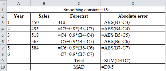
Forecast of sales using exponential smoothing with smoothing constant 0.9:
Given information:
| Year | Sales |
| 1 | 450 |
| 2 | 495 |
| 3 | 518 |
| 4 | 563 |
| 5 | 584 |
Formula to calculate the forecasted demand:
Where,
| Smoothing constant=0.9 | |||
| Year | Sales | Forecast | Absolute error |
| 1 | 450 | 410 | 40 |
| 2 | 495 | 446 | 49 |
| 3 | 518 | 490.1 | 27.9 |
| 4 | 563 | 515.21 | 47.79 |
| 5 | 584 | 558.221 | 25.779 |
| 6 | 581.4221 | ||
| Total | 190.469 | ||
| MAD | 38.0938 | ||
Excel worksheet:
Calculation of the forecast for year 2:
To calculate the forecast for year 2, substitute the value of forecast of year 1, smoothing constant and difference of actual and forecasted demand in the above formula. The result of the forecast for year 2 is 446.
Calculation of the forecast for year 3:
To calculate the forecast for year 3, substitute the value of forecast of year 2, smoothing constant and difference of actual and forecasted demand in the above formula. The result of the forecast for year 3 is 490.1.
Calculation of the forecast for year 4:
To calculate the forecast for year 4, substitute the value of forecast of year 3, smoothing constant and difference of actual and forecasted demand in the above formula. The result of the forecast for year 4 is 515.21.
Calculation of the forecast for year 5:
To calculate the forecast for year 5, substitute the value of forecast of year 4, smoothing constant and difference of actual and forecasted demand in the above formula. The result of forecast for year 5 is 558.221.
Calculation of the forecast for year 6:
To calculate the forecast for year 6, substitute the value of forecast of year 5, smoothing constant and difference of actual and forecasted demand in the above formula. The result of forecast for year 6 is 581.42.
Calculation of MAD using exponential smoothing with smoothing constant α=0.9:
Formula to calculate the Mean Absolute Deviation:
Calculation of the absolute error for year 1:
The absolute error for year 1 is the modulus of the difference between 450 and 410, which corresponds to 40. Therefore, the absolute error for year 1 is 40.
Calculation of the absolute error for year 2:
The absolute error for year 2 is the modulus of the difference between 495 and 446, which corresponds to 49. Therefore, the absolute error for year 2 is 49.
Calculation of the absolute error for year 3:
The absolute error for year 3 is the modulus of the difference between 518and490.1, which corresponds to 27.9. Therefore, the absolute error for year 3 is 27.9.
Calculation of the absolute error for year 4:
The absolute error for year 4 is the modulus of the difference between 563and515.21, which corresponds to 4.254. Therefore, the absolute error for year 4 is 47.79.
Calculation of the absolute error for year 5:
The absolute error for year 5 is the modulus of the difference between 584and558.221, which corresponds to 25.779. Therefore, the absolute error for year 5 is 25.779.
Calculation of the Mean Absolute Deviation using exponential smoothing:
Upon the substitution of summation value of absolute error for 5 years, that is, 190.469 is divided by the number of years. That is, 5 yields MAD of 38.093.
The forecast of sales using exponential smoothing with 0.9 as smoothing constant is 581.4221 and MAD is 38.093.
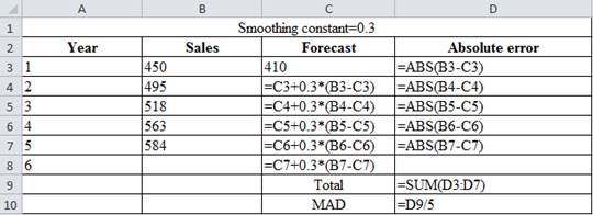
Forecast of sales using exponential smoothing with smoothing constant 0.3:
Given information:
| Year | Sales |
| 1 | 450 |
| 2 | 495 |
| 3 | 518 |
| 4 | 563 |
| 5 | 584 |
Formula to calculate the forecasted demand:
Where,
| Smoothing constant=0.3 | |||
| Year | Sales | Forecast | Absolute error |
| 1 | 450 | 410 | 40 |
| 2 | 495 | 422 | 73 |
| 3 | 518 | 443.9 | 74.1 |
| 4 | 563 | 466.13 | 96.87 |
| 5 | 584 | 495.191 | 88.809 |
| 6 | 521.8337 | ||
| Total | 372.779 | ||
| MAD | 74.5558 | ||
Excel worksheet:
Calculation of the forecast for year 2:
To calculate the forecast for year 2, substitute the value of forecast of year 1, smoothing constant and difference of actual and forecasted demand in the above formula. The result of the forecast for year 2 is 422.
Calculation of the forecast for year 3:
To calculate the forecast for year 3, substitute the value of forecast of year 2, smoothing constant and difference of actual and forecasted demand in the above formula. The result of the forecast for year 3 is 443.9.
Calculation of the forecast for year 4:
To calculate the forecast for year 4, substitute the value of forecast of year 3, smoothing constant and difference of actual and forecasted demand in the above formula. The result of the forecast for year 4 is 466.13.
Calculation of the forecast for year 5:
To calculate the forecast for year 5, substitute the value of forecast of year 4, smoothing constant and difference of actual and forecasted demand in the above formula. The result of the forecast for year 5 is 495.191.
Calculation of the forecast for year 6:
To calculate the forecast for year 6, substitute the value of forecast of year 5, smoothing constant and difference of actual and forecasted demand in the above formula. The result of the forecast for year 6 is 521.833.
Calculation of MAD using exponential smoothing with smoothing constant α=0.3:
Formula to calculate the Mean Absolute Deviation:
Calculation of the absolute error for year 1:
The absolute error for year 1 is the modulus of the difference between 450 and 410, which corresponds to 40. Therefore, the absolute error for year 1 is 40.
Calculation of the absolute error for year 2:
The absolute error for year 2 is the modulus of the difference between 495 and 422, which corresponds to 73. Therefore, the absolute error for year 2 is 73.
Calculation of the absolute error for year 3:
The absolute error for year 3 is the modulus of the difference between 518 and 443.9, which corresponds to 74.1. Therefore, the absolute error for year 3 is 74.1.
Calculation of the absolute error for year 4:
The absolute error for year 4 is the modulus of the difference between 563 and 466.13, which corresponds to 96.87. Therefore, the absolute error for year 4 is 96.87.
Calculation of the absolute error for year 5:
The absolute error for year 5 is the modulus of the difference between 584 and 495.191, which corresponds to 88.809. Therefore, the absolute error for year 5 is 88.809.
Calculation of the Mean Absolute Deviation using exponential smoothing with 0.3 as smoothing constant:
Upon the substitution of summation value of absolute error for 5 years, that is, 372.779 are divided by the number of years. That is, 5 yields MAD of 74.5558.
The forecast of sales using exponential smoothing with 0.3 as smoothing constant is 521.833 and MAD is 74.5558.
Hence, on comparing MAD from exponential smoothing with smoothing constant 0.3, 0.6 and 0.9 (refer to equations (1), (2) and (3)), it can be inferred that MAD of exponential smoothing with smoothing constant is most accurate because of least MAD.
Want to see more full solutions like this?
Chapter 4 Solutions
Pearson eText Principles of Operations Management: Sustainability and Supply Chain Management -- Instant Access (Pearson+)


- Communication Tips (2015) Tactful bragging Respond to the question "So, what do you do?" Whether you are student or have a job/internship, how can you tactfully brag in your answer to this question? Use the three elements from the video (listed below) when crafting your brag statement: Focus on results vs title Process vs job description Loop back to listener Example of an instructor's brag statement: "I help hundreds of students each semester to connect with one another, develop communication skills and prepare for upcoming interviews. Through improv games we explore presence, flexibility, and storytelling. How have your networking experiences on campus been so far?"arrow_forwardAccounting problemarrow_forwardGovernment's new plan to shift cargo from roads back to rail 26TH JANUARY 2024 Government is seeking to finalise a plan aimed at improving its rail network and move cargo away from a billion rand per day to its logistics crises, government has said an urgentturnaround is needed to improve its 31 000km locomotive network as more and more cargo moves from rail to trucks. The Department of Transport (DoT) hosted a discussion with industry stakeholders regarding the Freight Road to Rail Migration Plan on Thursday - the latest development in the wake of President Cyril Ramphosa forming the National Logistics Crisis Committee last year. Transnet, the South African National Roads Agency (Sanral) and private sector companies were all in attendance. The Freight Road to Rail Migration Plan is part of government's strategies to improve the country's ongoing logistics crises. In October last year, the government unveiled its Freight Logistics Roadmap to improve the ports and rail networks and…arrow_forward
- Assess what led to such logistical inefficiencies / collapse of a previously world class freight networkarrow_forwardWhich of the following statements concerning the evaluation of training programs is true? Most companies thoroughly evaluate the return on investment of their training programs It is relatively easy to establish a control group and a treatment group for evaluation Results level of evaluation measures how well participants liked the program Behavior level criteria measure whether skills learned in training result in behavior changes back on the jobarrow_forwardEligibility testing is an disparate impact validation method none of the above a method to validate promotions and progressive discipline activity a test an employee administers to ensure that the potential employee is capable and qualified to perform the requirements of the positionarrow_forward
- A no-strike pledge by a union in a collective bargaining agreement is given in return for management’s agreement to: a grievance procedure a union shop a wage increase a fringe benefit increase binding arbitration of grievancesarrow_forwardWhich is the major OD technique that is used for increasing the communication, cooperation, and cohesiveness of work units? Leadership analysis Developing objectives Groupthink Strategic Planning team Buildingarrow_forwardAn American multinational firm usually is less than fully successful in adapting itself to local practices in each country because: American managers are often ignorant of local conditions None of the above management direction may be centralized in the home office All of the above Foreign subsidiaries often have American managersarrow_forward
- When salary increases are based on inputs, or performance, companies are following: agency theory equality theory equity theory compliance theory need theoryarrow_forwardThe most frequently used techniques for measuring job satisfaction involves Direct observation Questionnaires Interviews Psychological testsarrow_forwardWhich of the following is not an advantage of on-the-job training? Transfer is less difficult Transfer is less difficult The training is inexpensive Any organizational member can be the trainer without preparation It is relatively easy to use this methodarrow_forward
 Contemporary MarketingMarketingISBN:9780357033777Author:Louis E. Boone, David L. KurtzPublisher:Cengage Learning
 MarketingMarketingISBN:9780357033791Author:Pride, William MPublisher:South Western Educational Publishing
 Practical Management ScienceOperations ManagementISBN:9781337406659Author:WINSTON, Wayne L.Publisher:Cengage,