
Concept explainers
Videos
At you can see in the following table, demand for heart transplant surgery at Washington General Hospital has increased steadily in the past few years:
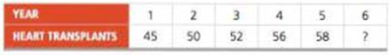
The director of medical services predicted 6 years ago that demand in year 1 would be 41 surgeries.
a) Use exponential smoothing, first with a smoothing constant of .6 and then with one of .9, to develop forecasts for years 2 through 6.
b) Use a 3-year moving average to forecast demand in years 4, 5, and 6.
c) Use the trend-projection method to forecast demand in years 1 through 6.
d) With MAD as the criterion, which of the four
a)
To determine: Findthe forecast for years 2 through 6, using exponential smoothing.
Introduction: A sequence of data pointing in successive order is known as time series. Time series forecasting is the prediction based on past events which are at a uniform time interval. Moving average method and trend projections are one of the time series methods which use weights to prioritize past data.
Answer to Problem 13P
The forecast for years 2 through 6 using exponential smoothing with smoothing constant 0.6 is 56.263 and smoothing constant 0.9 is 57.757.
Explanation of Solution
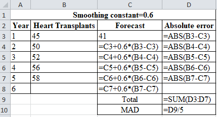
Forecast for years 1 through 6 using exponential smoothing with smoothing constant 0.6:
Given information:
| Year | 1 | 2 | 3 | 4 | 5 | 6 |
| Heart Transplants | 45 | 50 | 52 | 56 | 58 |
Formula to calculate the forecasted demand:
Where,
| Smoothing constant=0.6 | |||
| Year | Heart Transplants | Forecast | Absolute error |
| 1 | 45 | 41 | 4.000 |
| 2 | 50 | 43.400 | 6.600 |
| 3 | 52 | 47.360 | 4.640 |
| 4 | 56 | 50.144 | 5.856 |
| 5 | 58 | 53.658 | 4.342 |
| 6 | 56.263 | ||
| Total | 25.438 | ||
| MAD | 5.08768 | ||
Excel worksheet:
Calculation of the forecast for year 2:
To calculate forecast for year 2, substitute the value of forecast of year 1, smoothing constant and difference of actual and forecasted demand in the above formula. The result of the forecast for year 2 is 43.40.
Calculation of the forecast for year 3:
To calculate forecast for year 3, substitute the value of forecast of year 2, smoothing constant and difference of actual and forecasted demand in the above formula. The result of the forecast for year 3 is 47.360.
Calculation of the forecast for year 4:
To calculate forecast for year 4, substitute the value of forecast of year 3, smoothing constant and difference of actual and forecasted demand in the above formula. The result of the forecast for year 4 is 50.144.
Calculation of the forecast for year 5:
To calculate forecast for year 5, substitute the value of forecast of year 4, smoothing constant and difference of actual and forecasted demand in the above formula. The result of the forecast for year 5 is 53.658.
Calculation of the forecast for year 6:
To calculate forecast for year 6, substitute the value of forecast of year 5, smoothing constant and difference of actual and forecasted demand in the above formula. The result of the forecast for year 6 is 56.263.
Calculation of MAD using exponential smoothing with smoothing constant α=0.6:
Formula to calculate the Mean Absolute Deviation:
Calculation of the absolute error for year 1:
The absolute error for year 1 is the modulus of the difference between 45 and 41, which corresponds to 4. Therefore, the absolute error for year 1 is 4.
Calculation of the absolute error for year 2:
The absolute error for year 2 is the modulus of the difference between 50 and 43.4, which corresponds to 6.6. Therefore, the absolute error for year 2 is 6.6.
Calculation of the absolute error for year 3:
The absolute error for year 3 is the modulus of the difference between 52 and 47.360, which corresponds to 4.640. Therefore, the absolute error for year 3 is4.640.
Calculation of the absolute error for year 4:
The absolute error for year 4 is the modulus of the difference between 56 and 50.144, which corresponds to 5.856. Therefore, the absolute error for year 4 is5.856.
Calculation of the absolute error for year 5:
The absolute error for year 5 is the modulus of the difference between 58 and 53.658, which corresponds to 4.342. Therefore, the absolute error for year 5 is 4.342.
Calculation of the Mean Absolute Deviation using exponential smoothing:
Upon the substitution of summation value of absolute error for 5 years, that is, 25.438 are divided by number of years. That is, 5 yields MAD of 5.08768.
The forecast for years 2 through 6 using exponential smoothing with 0.6 as smoothing constant is 56.263.
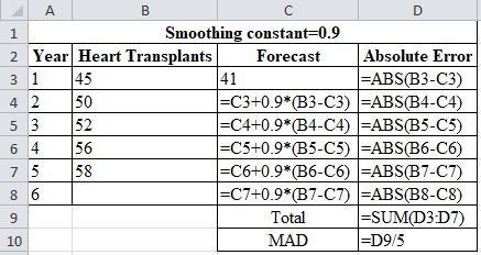
The forecast for years 1 through 6 using exponential smoothing with smoothing constant 0.9:
Given information:
| Year | 1 | 2 | 3 | 4 | 5 | 6 |
| Heart Transplants | 45 | 50 | 52 | 56 | 58 |
Formula to calculate the forecasted demand:
Where
| Smoothing constant=0.9 | |||
| Year | Heart Transplants | Forecast | Absolute Error |
| 1 | 45 | 41 | 4 |
| 2 | 50 | 44.600 | 5.400 |
| 3 | 52 | 49.460 | 2.540 |
| 4 | 56 | 51.746 | 4.254 |
| 5 | 58 | 55.575 | 2.425 |
| 6 | 57.757 | 57.757 | |
| Total | 18.6194 | ||
| MAD | 3.72388 | ||
Excel worksheet:
Calculation of the forecast for year 2:
To calculate the forecast for year 2, substitute the value of forecast of year 1, smoothing constant and difference of actual and forecasted demand in the above formula. The result of the forecast for year 2 is 44.60.
Calculation of the forecast for year 3:
To calculate forecast for year 3, substitute the value of forecast of year 2, smoothing constant and difference of actual and forecasted demand in the above formula. The result of the forecast for year 3 is 49.460.
Calculation of the forecast for year 4:
To calculate forecast for year 4, substitute the value of forecast of year 3, smoothing constant and difference of actual and forecasted demand in the above formula. The result of the forecast for year 4 is 50.144.
Calculation of the forecast for year 5:
To calculate forecast for year 5, substitute the value of forecast of year 4, smoothing constant and difference of actual and forecasted demand in the above formula. The result of the forecast for year 5 is55.575.
Calculation of the forecast for year 6:
To calculate forecast for year 6, substitute the value of forecast of year 5, smoothing constant and difference of actual and forecasted demand in the above formula. The result of the forecast for year 6 is57.757.
Calculation of MAD using exponential smoothing with smoothing constant α=0.9:
Formula to calculate the Mean Absolute Deviation:
Calculation of the absolute error for year 1:
The absolute error for year 1 is the modulus of the difference between 45 and 41, which corresponds to 4. Therefore, the absolute error for year 1 is 4.
Calculation of the absolute error for year 2:
The absolute error for year 2 is the modulus of the difference between 50 and 44.6, which corresponds to 5.4. Therefore, the absolute error for year 2 is 5.4.
Calculation of the absolute error for year 3:
The absolute error for year 3 is the modulus of the difference between 52 and49.460, which corresponds to 2.540. Therefore, the absolute error for year 3 is2.540.
Calculation of the absolute error for year 4:
The absolute error for year 4 is the modulus of the difference between 56 and51.746, which corresponds to 4.254. Therefore, the absolute error for year 4 is4.254.
Calculation of the absolute error for year 5:
The absolute error for year 5 is the modulus of the difference between 58 and55.575, which corresponds to 2.425. Therefore, the absolute error for year 5 is 2.425.
Calculation of the Mean Absolute Deviation using exponential smoothing:
Upon the substitution of summation value of absolute error for 5 years, that is,18.6194are divided by the number of years. That is, 5 yields MAD of 3.72388.
The forecast for years 2 through 6 using exponential smoothing with 0.9 as smoothing constant is 57.757.
Hence, the forecast for years 2 through 6 using exponential smoothing with smoothing constant 0.6 is 56.263 and smoothing constant 0.9 is 57.757.
b)
To determine: Using 3-year moving average, forecast the demand for years 4, 5 and 6.
Answer to Problem 13P
The demand forecast for years 4, 5 and 6 is 49, 52.67 and 55.33.
Explanation of Solution
Given information:
| Year | 1 | 2 | 3 | 4 | 5 | 6 |
| Heart Transplants | 45 | 50 | 52 | 56 | 58 |
Formula to calculate the forecasted demand:
| Year | Heart Transplants | Forecast | Absolute Error |
| 1 | 45 | ||
| 2 | 50 | ||
| 3 | 52 | ||
| 4 | 56 | 49 | 7 |
| 5 | 58 | 52.67 | 5.333 |
| 6 | 55.33 | ||
| Total | 12.333 | ||
| MAD | 6.1667 |
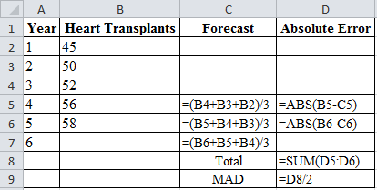
Excel worksheet:
Calculation of the forecast for year 4:
To calculate the forecast for year 4, divide the summation of the values from years 1, 2 and 3 and divide by 3. The corresponding value 49 is the forecast for year 4. The 3-year moving average for year 4 is 49.
Calculation of the forecast for year 5:
To calculate the forecast for year 5, divide the summation of the values from years 2, 3 and 4 and divide by 3. The corresponding value 52.67 is the forecast for year 5. The 3-year moving average for year 5 is 52.67.
Calculation of the forecast for year 6:
To calculate the forecast for year 6, divide the summation of the values from years 3, 4, 5 and divide by 3. The corresponding value 55.33 is the forecast for year 5. The 3-year moving average for year 5 is 55.33.
Calculation of MAD using 3-year moving average:
Formula to calculate the Mean Absolute Deviation:
Calculation of the absolute error for year 4:
The absolute error for year 4 is the modulus of the difference between 56 and 49, which corresponds to 7. Therefore, the absolute error for year 4 is 7.
Calculation of the absolute error for year 5:
The absolute error for year 4 is the modulus of the difference between 58 and 52.67, which corresponds to 5.33. Therefore, the absolute error for year 4 is 5.33.
Calculation of the Mean Absolute Deviation using 3-year moving average:
Upon the substitution of the summation value of the absolute error for 2 years, that is,12.333is divided by number of years. That is, 2 yields MAD of 6.1666.
Hence, the demand forecast for years 4, 5 and 6 is 49, 52.67 and 55.33.
c)
To determine: Find the demand forecast in year 1 through 6using trend projection.
Answer to Problem 13P
The forecast in year 1 through 6using trend projection is62.1.
Explanation of Solution
Given information:
| Year | 1 | 2 | 3 | 4 | 5 | 6 |
| Heart Transplants | 45 | 50 | 52 | 56 | 58 |
Formula to calculate the demand forecast
Where,
Where,
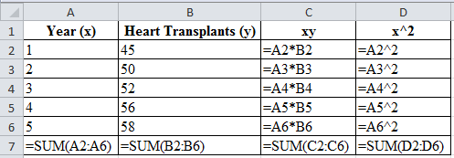
| Year (x) | Heart Transplants (y) | xy | x^2 |
| 1 | 45 | 45 | 1 |
| 2 | 50 | 100 | 4 |
| 3 | 52 | 156 | 9 |
| 4 | 56 | 224 | 16 |
| 5 | 58 | 290 | 25 |
| ∑=15 | ∑=261 | ∑=815 | ∑=55 |
Excel worksheet
Substituting the values in the above formula
Calculation of average of x values
The average of x values is obtained by dividing the summation of x values, that is, (1+2+…+5) with the number of period n. That is, 5. The value of
Calculation of average of y values
The average of y values is obtained by dividing the summation of sales with the number of period n. That is, 5. The value of
Calculation of slope of regression line‘b’:
The summation of product of sales (y) with x values is ∑xy = 815, the product of number of years (n), the average of x values and the average of y values is obtained. That is,
The summation of square of x values, that is, 55 is subtracted from the product of the number of years. That is,5 with average of x values;3. The resultant value is 10. The slope of regression line is obtained by dividing 32 with 10. The value of ‘b’ is 3.2.
Calculation of y-axis intercept ‘a’:
The y-axis intercept is obtained by the difference between average of y values and values obtained by the product of slope of regression line with average of x values. The resultant value of ‘a’ is 42.9.
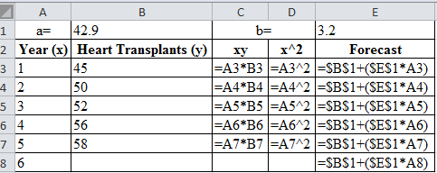
Calculation of the forecast for years 1 through 6:
| a= | 42.9 | b= | 3.2 | |
| Year (x) | Heart Transplants (y) | xy | x^2 | Forecast |
| 1 | 45 | 45 | 1 | 46.1 |
| 2 | 50 | 100 | 4 | 49.3 |
| 3 | 52 | 156 | 9 | 52.5 |
| 4 | 56 | 224 | 16 | 55.7 |
| 5 | 58 | 290 | 25 | 58.9 |
| 6 | 62.1 | |||
Excel worksheet:
Calculation of forecast of year 1:
The forecast for year 1 is obtained by the summation of the product of slope of regression line and forecasted year, with the y-axis intercept. The forecasted value obtained is 46.1.
Calculation of forecast of year 2:
The forecast for year 2 is obtained by the summation of the product of slope of regression line and forecasted year, with the y-axis intercept. The forecasted value obtained is 49.3.
Calculation of forecast of year 3:
The forecast for year 3 is obtained by the summation of the product of slope of regression line and forecasted year, with the y-axis intercept. The forecasted value obtained is 52.5.
Calculation of forecast of year 4:
The forecast for year 4 is obtained by the summation of the product of slope of regression line and forecasted year, with the y-axis intercept. The forecasted value obtained is 55.7.
Calculation of forecast of year 5:
The forecast for year 5 is obtained by the summation of the product of slope of regression line and forecasted year, with the y-axis intercept. The forecasted value obtained is 58.9.
Calculation of forecast of year 6:
The forecast for year 6 is obtained by the summation of the product of slope of regression line and forecasted year, with the y-axis intercept. The forecasted value obtained is 62.1.
Formula to calculate the Mean Absolute Deviation:
Calculation of MAD using trend projection:
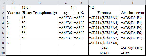
| a= | 42.9 | b= | 3.2 | ||
| Year (x) | Heart Transplants (y) | xy | x^2 | Forecast | Absolute error |
| 1 | 45 | 45 | 1 | 46.1 | 1.1 |
| 2 | 50 | 100 | 4 | 49.3 | 0.7 |
| 3 | 52 | 156 | 9 | 52.5 | 0.5 |
| 4 | 56 | 224 | 16 | 55.7 | 0.3 |
| 5 | 58 | 290 | 25 | 58.9 | 0.9 |
| 6 | 62.1 | ||||
| Total | 3.5 | ||||
| MAD | 0.7 | ||||
Excel worksheet:
Calculation of the absolute error for year 1:
The absolute error for year 1 is the modulus of the difference between 45 and 46.1, which corresponds to 1.1. Therefore, the absolute error for year 1 is 1.1.
Calculation of the absolute error for year 2:
The absolute error for year 2 is the modulus of the difference between 50 and 49.3, which corresponds to 0.7. Therefore, the absolute error for year 2 is 0.7.
Calculation of the absolute error for year 3:
The absolute error for year 3 is the modulus of the difference between 52 and 52.5, which corresponds to 0.5. Therefore, the absolute error for year 3 is 0.5.
Calculation of the absolute error for year 4:
The absolute error for year 4 is the modulus of the difference between 56 and 55.7, which corresponds to 0.3. Therefore, the absolute error for year 4 is 0.3.
Calculation of the absolute error for year 5:
The absolute error for year 5 is the modulus of the difference between 58 and 58.9, which corresponds to 0.9. Therefore, the absolute error for year 5 is 0.9.
Calculation of the Mean Absolute Deviation using trend projection:
Upon the substitution of summation value of absolute error for 5 years, that is,3.5is divided by the number of years. That is,5 yields MAD of 0.7.
Thus, the forecast in year 1 through 6 using trend projection is 62.1.
d)
To determine: Compare the MAD of exponential smoothing, 3-year moving average and trend projection and infer the best method.
Explanation of Solution
On Comparing MAD from the four methods, (refer to equations (1), (2), (3) and (4)) it can be inferred that trend projection is the best methods since it has the least MAD.
Want to see more full solutions like this?
Chapter 4 Solutions
Pearson eText Principles of Operations Management: Sustainability and Supply Chain Management -- Instant Access (Pearson+)


- EXPLAIN Human Resource Information System (HRIS)arrow_forwardRead the mini-case study below and answer the following questions.With an enormous amount of data stored in databases and data warehouses, it is increasinglyimportant to develop powerful tools for analysis of such data and mining interestingknowledge from it. Data mining is a process of inferring knowledge from such huge data. Themain problem related to the retrieval of information from the World Wide Web is theenormous number of unstructured documents and resources, i.e., the difficulty of locating andtracking appropriate sources.Briefly explain any five (5) types of information you can get from data mining.arrow_forwardProblem 1: Practice Problems Chapter 6 Managing Quality The accounts receivable department has documented the following defects over a 30-day period: Category Frequency Invoice amount does not agree with the check amount 108 Invoice not on record (not found) 24 No formal invoice issued Check (payment) not received on time 18 30 Check not signed 8 Invoice number and invoice referenced do not agree 12 What techniques would you use and what conclusions can you draw about defects in the accounts receivable department? Problem 2: Prepare a flow chart for purchasing a Big Mac at the drive-through window at McDonalds. Problem 3: Draw a fishbone chart detailing reasons why a part might not be correctly machined.arrow_forward
- Problem 5: Development of a new deluxe version of a particular software product is being considered. The activities necessary for the completion of this project are listed in the table below along with their costs and completion times in weeks. Activity Normal Crash Normal Crash Immediate Time Time Cost Cost Predecessor A 4 3 2,000 2,600 B 2 1 2,200 2,800 A C 3 3 500 500 A D 8 4 2,300 2,600 A E 6 3 900 1,200 B, D F 3 2 3,000 4,200 C, E G 4 2 1,400 2,000 F a. What is the project expected completion date? b. What is the total cost required for completing this project on normal time? c. If you wish to reduce the time required to complete this project by 1 week, which activity should be crashed, and how much will this increase the total cost?arrow_forwardI need answer typing clear urjent no chatgpt used pls i will give 5 Upvotes.with diagramarrow_forwardnot use ai pleasearrow_forward
- provide scholarly reseach and references for the following 1. explain operational risks and examples of such risk faced by management at financial institutions 2. discuss the importance of establishing an effective risk management policy at financial institutions to manage operational risk, giving example of a risk management strategy used by financial institutions to mitigate such risk. 3. what is the rold of the core principles of effective bank supervision as it relates to operational risk, in the effective management of financial institutions.arrow_forwardPlease show all units, work, and steps needed to solve this problem I need answer typing clear urjent no chatgpt used pls i will give 5 Upvotes.arrow_forwardIM.82 A distributor of industrial equipment purchases specialized compressors for use in air conditioners. The regular price is $50, however, the manufacturer of this compressor offers quantity discounts per the following discount schedule: Option Plan Quantity Discount A 1 - 299 0% B 300 - 1,199 0.50% C 1,200+ 1.50% The distributor pays $56 each time it places an order with the manufacturer. Holding costs are negligible (none) but they do earn 10% annual interest on all cash balances (meaning there will be a financial opportunity cost when they put cash into inventory). Annual demand is expected to be 10,750 units. When there is no quantity discount (Option Plan A, the first row of the schedule listed above), what is the adjusted order quantity? (Display your answer to the nearest whole number.) 491 Based on your answer to the previous question, and based on the annual demand as stated above, what will be the annual ordering costs? (Display your answer to the…arrow_forward
- Excel Please. The workload of many areas of banking operations varies considerably based on time of day. A variable capacity can be achieved effectively by employing part-time personnel. Because part-timers are not entitled to all the fringe benefits, they are often more economical than full-time employees. Other considerations, however, may limit the extent to which part-time people can be hired in a given department. The problem is to find an optimal workforce schedule that would meet personnel requirements at any given time and also be economical. Some of the factors affecting personnel assignments are listed here: The bank is open from 9:00am to 7:00pm. Full-time employees work for 8 hours (1 hour for lunch included) per day. They do not necessarily have to start their shift when the bank opens. Part-time employees work for at least 4 hours per day, but less than 8 hours per day and do not get a lunch break. By corporate policy, total part-time personnel hours is limited…arrow_forwardIM.84 An outdoor equipment manufacturer sells a rugged water bottle to complement its product line. They sell this item to a variety of sporting goods stores and other retailers. The manufacturer offers quantity discounts per the following discount schedule: Option Plan Quantity Price A 1 - 2,399 $5.50 B 2,400 - 3,999 $5.20 C 4,000+ $4.50 A large big-box retailer expects to sell 9,700 units this year. This retailer estimates that it incurs an internal administrative cost of $225 each time it places an order with the manufacturer. Holding cost for the retailer is $55 per case per year. (There are 40 units or water bottles per case.) Based on this information, and not taking into account any quantity discount offers, what is the calculated EOQ (in units)? (Display your answer to the nearest whole number.) Number Based on this information, sort each quantity discount plan from left to right by dragging the MOST preferred option plan to the left, and the LEAST preferred…arrow_forwardIn less than 150 words, what is an example of what your reflection of core values means to you and your work: Commitment, Perseverance, Community, Service, Pride?arrow_forward
 Contemporary MarketingMarketingISBN:9780357033777Author:Louis E. Boone, David L. KurtzPublisher:Cengage Learning
 MarketingMarketingISBN:9780357033791Author:Pride, William MPublisher:South Western Educational Publishing
 Practical Management ScienceOperations ManagementISBN:9781337406659Author:WINSTON, Wayne L.Publisher:Cengage,
 Purchasing and Supply Chain ManagementOperations ManagementISBN:9781285869681Author:Robert M. Monczka, Robert B. Handfield, Larry C. Giunipero, James L. PattersonPublisher:Cengage Learning