
Concept explainers
Videos
Relationship between body weight and backpack weight for this group of hikers.
Answer to Problem 7E
Linear, positive, and moderately strong association with one outlier.
Explanation of Solution
Given information:
For
On horizontal axis: Body weight
On vertical axis: Backpack weight
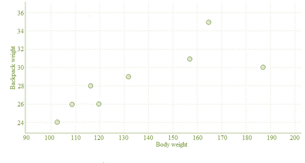
Strength: In the scatterplot, the points do not lie very close together and do not spread far apart as well. Thus, strength will be moderately strong.
Form: In the scatterplot, no strong curvature exists. Thus, form will be linear.
Direction: Due to the upward slope of the pattern, the direction will be positive.
Unusual features: In the scatterplot, rightmost point appears to deviate significantly from the general linear pattern in the other points. Thus, one outlier exists.
Chapter 3 Solutions
PRACTICE OF STATISTICS F/AP EXAM
Additional Math Textbook Solutions
University Calculus: Early Transcendentals (4th Edition)
College Algebra (7th Edition)
A Problem Solving Approach To Mathematics For Elementary School Teachers (13th Edition)
College Algebra with Modeling & Visualization (5th Edition)
Algebra and Trigonometry (6th Edition)
Elementary Statistics (13th Edition)


- 4. Dynamic regression (adapted from Q10.4 in Hyndman & Athanasopoulos) This exercise concerns aus_accommodation: the total quarterly takings from accommodation and the room occupancy level for hotels, motels, and guest houses in Australia, between January 1998 and June 2016. Total quarterly takings are in millions of Australian dollars. a. Perform inflation adjustment for Takings (using the CPI column), creating a new column in the tsibble called Adj Takings. b. For each state, fit a dynamic regression model of Adj Takings with seasonal dummy variables, a piecewise linear time trend with one knot at 2008 Q1, and ARIMA errors. c. What model was fitted for the state of Victoria? Does the time series exhibit constant seasonality? d. Check that the residuals of the model in c) look like white noise.arrow_forwardce- 216 Answer the following, using the figures and tables from the age versus bone loss data in 2010 Questions 2 and 12: a. For what ages is it reasonable to use the regression line to predict bone loss? b. Interpret the slope in the context of this wolf X problem. y min ball bas oft c. Using the data from the study, can you say that age causes bone loss? srls to sqota bri vo X 1931s aqsini-Y ST.0 0 Isups Iq nsalst ever tom vam noboslios tsb a ti segood insvla villemari aixs-Yediarrow_forward120 110 110 100 90 80 Total Score Scatterplot of Total Score vs. Putts grit bas 70- 20 25 30 35 40 45 50 Puttsarrow_forward
- 10 15 Answer the following, using the figures and tables from the temperature versus coffee sales data from Questions 1 and 11: a. How many coffees should the manager prepare to make if the temperature is 32°F? b. As the temperature drops, how much more coffee will consumers purchase?ov (Hint: Use the slope.) 21 bru sug c. For what temperature values does the voy marw regression line make the best predictions? al X al 1090391-Yrit,vewolf 30-X Inlog arts bauoxs 268 PART 4 Statistical Studies and the Hunt forarrow_forward18 Using the results from the rainfall versus corn production data in Question 14, answer DOV 15 the following: a. Find and interpret the slope in the con- text of this problem. 79 b. Find the Y-intercept in the context of this problem. alb to sig c. Can the Y-intercept be interpreted here? (.ob or grinisiques xs as 101 gniwollol edt 958 orb sz) asiques sich ed: flow wo PEMAIarrow_forwardVariable Total score (Y) Putts hit (X) Mean. 93.900 35.780 Standard Deviation 7.717 4.554 Correlation 0.896arrow_forward
- 17 Referring to the figures and tables from the golf data in Questions 3 and 13, what hap- pens as you keep increasing X? Does Y increase forever? Explain. comis word ே om zol 6 svari woy wol visy alto su and vibed si s'ablow it bas akiog vino b tad) beil Bopara Aon csu How wod griz -do 30 義arrow_forwardVariable Temperature (X) Coffees sold (Y) Mean 35.08 29,913 Standard Deviation 16.29 12,174 Correlation -0.741arrow_forward13 A golf analyst measures the total score and number of putts hit for 100 rounds of golf an amateur plays; you can see the summary of statistics in the following table. (See the figure in Question 3 for a scatterplot of this data.)noitoloqpics bella a. Is it reasonable to use a line to fit this data? Explain. 101 250 b. Find the equation of the best fitting 15er regression line. ad aufstuess som 'moob Y lo esulav in X ni ognado a tad Variable on Mean Standard Correlation 92 Deviation Total score (Y) 93.900 7.717 0.896 Putts hit (X) 35.780 4.554 totenololbenq axlam riso voy X to asulisy datdw gribol anil er 08,080.0 zl noitsism.A How atharrow_forward
- Variable Bone loss (Y) Age (X) Mean 35.008. 67.992 Standard Deviation 7.684 10.673 Correlation 0.574arrow_forward50 Bone Loss 30 40 20 Scatterplot of Bone Loss vs. Age . [902) 10 50 60 70 80 90 Age a sub adi u xinq (20) E 4 adw I- nyd med ivia .0 What does a scatterplot that shows no linear relationship between X and Y look like?arrow_forwardVariable Temperature (X) Coffees sold (Y) Mean 35.08 29,913 Standard Deviation 16.29 12,174 Correlation -0.741arrow_forward
 MATLAB: An Introduction with ApplicationsStatisticsISBN:9781119256830Author:Amos GilatPublisher:John Wiley & Sons Inc
 Probability and Statistics for Engineering and th...StatisticsISBN:9781305251809Author:Jay L. DevorePublisher:Cengage Learning
 Statistics for The Behavioral Sciences (MindTap C...StatisticsISBN:9781305504912Author:Frederick J Gravetter, Larry B. WallnauPublisher:Cengage Learning
 Elementary Statistics: Picturing the World (7th E...StatisticsISBN:9780134683416Author:Ron Larson, Betsy FarberPublisher:PEARSON
 The Basic Practice of StatisticsStatisticsISBN:9781319042578Author:David S. Moore, William I. Notz, Michael A. FlignerPublisher:W. H. Freeman
 Introduction to the Practice of StatisticsStatisticsISBN:9781319013387Author:David S. Moore, George P. McCabe, Bruce A. CraigPublisher:W. H. Freeman