
Videos
(a)
To make a
(a)
Explanation of Solution
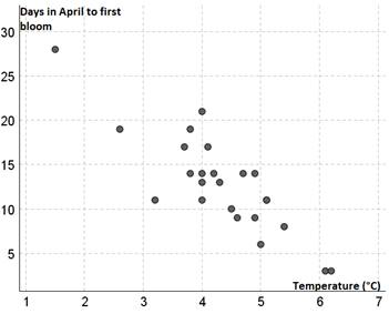
Since we expect the temperature to influence the days in April to first blossom temperature is the explanatory variable and the days in April to first blossom is the response variable. Thus, the scatterplot is as:
(b)
To use the technology to calculate the
(b)
Answer to Problem R3.4RE
Explanation of Solution
Using calculator, press on STAT and then select
Next, press on STAT select CALC and then select
Finally, pressing on ENTER then gives us the following result:
This then implies the regression line as:
This then implies that on average, the days in April to first blossom decreases by
(c)
To explain would you be willing to use the equation in part (b) to predict the date of the first blossom.
(c)
Answer to Problem R3.4RE
No.
Explanation of Solution
The regression line in part (b) is:
To predict the date to first blossom at
We then note that the predicted day to first blossom in April is
(d)
To calculate and interpret the residual for the year when the average March temperature was
(d)
Answer to Problem R3.4RE
Residual is
Explanation of Solution
The regression line in part (b) is:
Now, the days to first blossom when average March temperature was
And the actual value is
Thus, the residual is as:
This then implies that we overestimated the number of days in April to first blossom by
(e)
To use the technology to help construct the residual plot and describe what you see.
(e)
Explanation of Solution
The residual plot is as:
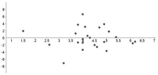
Thus, there is no obvious pattern in the residual plot and thus the linear regression line seems to be a good fit.
Chapter 3 Solutions
PRACTICE OF STATISTICS F/AP EXAM
Additional Math Textbook Solutions
College Algebra (7th Edition)
Elementary Statistics (13th Edition)
Pre-Algebra Student Edition
University Calculus: Early Transcendentals (4th Edition)
Calculus: Early Transcendentals (2nd Edition)


- Business discussarrow_forwardSpam filters are built on principles similar to those used in logistic regression. We fit a probability that each message is spam or not spam. We have several variables for each email. Here are a few: to_multiple=1 if there are multiple recipients, winner=1 if the word 'winner' appears in the subject line, format=1 if the email is poorly formatted, re_subj=1 if "re" appears in the subject line. A logistic model was fit to a dataset with the following output: Estimate SE Z Pr(>|Z|) (Intercept) -0.8161 0.086 -9.4895 0 to_multiple -2.5651 0.3052 -8.4047 0 winner 1.5801 0.3156 5.0067 0 format -0.1528 0.1136 -1.3451 0.1786 re_subj -2.8401 0.363 -7.824 0 (a) Write down the model using the coefficients from the model fit.log_odds(spam) = -0.8161 + -2.5651 + to_multiple + 1.5801 winner + -0.1528 format + -2.8401 re_subj(b) Suppose we have an observation where to_multiple=0, winner=1, format=0, and re_subj=0. What is the predicted probability that this message is spam?…arrow_forwardConsider an event X comprised of three outcomes whose probabilities are 9/18, 1/18,and 6/18. Compute the probability of the complement of the event. Question content area bottom Part 1 A.1/2 B.2/18 C.16/18 D.16/3arrow_forward
- John and Mike were offered mints. What is the probability that at least John or Mike would respond favorably? (Hint: Use the classical definition.) Question content area bottom Part 1 A.1/2 B.3/4 C.1/8 D.3/8arrow_forwardThe details of the clock sales at a supermarket for the past 6 weeks are shown in the table below. The time series appears to be relatively stable, without trend, seasonal, or cyclical effects. The simple moving average value of k is set at 2. What is the simple moving average root mean square error? Round to two decimal places. Week Units sold 1 88 2 44 3 54 4 65 5 72 6 85 Question content area bottom Part 1 A. 207.13 B. 20.12 C. 14.39 D. 0.21arrow_forwardThe details of the clock sales at a supermarket for the past 6 weeks are shown in the table below. The time series appears to be relatively stable, without trend, seasonal, or cyclical effects. The simple moving average value of k is set at 2. If the smoothing constant is assumed to be 0.7, and setting F1 and F2=A1, what is the exponential smoothing sales forecast for week 7? Round to the nearest whole number. Week Units sold 1 88 2 44 3 54 4 65 5 72 6 85 Question content area bottom Part 1 A. 80 clocks B. 60 clocks C. 70 clocks D. 50 clocksarrow_forward
- The details of the clock sales at a supermarket for the past 6 weeks are shown in the table below. The time series appears to be relatively stable, without trend, seasonal, or cyclical effects. The simple moving average value of k is set at 2. Calculate the value of the simple moving average mean absolute percentage error. Round to two decimal places. Week Units sold 1 88 2 44 3 54 4 65 5 72 6 85 Part 1 A. 14.39 B. 25.56 C. 23.45 D. 20.90arrow_forwardThe accompanying data shows the fossil fuels production, fossil fuels consumption, and total energy consumption in quadrillions of BTUs of a certain region for the years 1986 to 2015. Complete parts a and b. Year Fossil Fuels Production Fossil Fuels Consumption Total Energy Consumption1949 28.748 29.002 31.9821950 32.563 31.632 34.6161951 35.792 34.008 36.9741952 34.977 33.800 36.7481953 35.349 34.826 37.6641954 33.764 33.877 36.6391955 37.364 37.410 40.2081956 39.771 38.888 41.7541957 40.133 38.926 41.7871958 37.216 38.717 41.6451959 39.045 40.550 43.4661960 39.869 42.137 45.0861961 40.307 42.758 45.7381962 41.732 44.681 47.8261963 44.037 46.509 49.6441964 45.789 48.543 51.8151965 47.235 50.577 54.0151966 50.035 53.514 57.0141967 52.597 55.127 58.9051968 54.306 58.502 62.4151969 56.286…arrow_forwardThe accompanying data shows the fossil fuels production, fossil fuels consumption, and total energy consumption in quadrillions of BTUs of a certain region for the years 1986 to 2015. Complete parts a and b. Year Fossil Fuels Production Fossil Fuels Consumption Total Energy Consumption1949 28.748 29.002 31.9821950 32.563 31.632 34.6161951 35.792 34.008 36.9741952 34.977 33.800 36.7481953 35.349 34.826 37.6641954 33.764 33.877 36.6391955 37.364 37.410 40.2081956 39.771 38.888 41.7541957 40.133 38.926 41.7871958 37.216 38.717 41.6451959 39.045 40.550 43.4661960 39.869 42.137 45.0861961 40.307 42.758 45.7381962 41.732 44.681 47.8261963 44.037 46.509 49.6441964 45.789 48.543 51.8151965 47.235 50.577 54.0151966 50.035 53.514 57.0141967 52.597 55.127 58.9051968 54.306 58.502 62.4151969 56.286…arrow_forward
- The accompanying data shows the fossil fuels production, fossil fuels consumption, and total energy consumption in quadrillions of BTUs of a certain region for the years 1986 to 2015. Complete parts a and b. Develop line charts for each variable and identify the characteristics of the time series (that is, random, stationary, trend, seasonal, or cyclical). What is the line chart for the variable Fossil Fuels Production?arrow_forwardThe accompanying data shows the fossil fuels production, fossil fuels consumption, and total energy consumption in quadrillions of BTUs of a certain region for the years 1986 to 2015. Complete parts a and b. Year Fossil Fuels Production Fossil Fuels Consumption Total Energy Consumption1949 28.748 29.002 31.9821950 32.563 31.632 34.6161951 35.792 34.008 36.9741952 34.977 33.800 36.7481953 35.349 34.826 37.6641954 33.764 33.877 36.6391955 37.364 37.410 40.2081956 39.771 38.888 41.7541957 40.133 38.926 41.7871958 37.216 38.717 41.6451959 39.045 40.550 43.4661960 39.869 42.137 45.0861961 40.307 42.758 45.7381962 41.732 44.681 47.8261963 44.037 46.509 49.6441964 45.789 48.543 51.8151965 47.235 50.577 54.0151966 50.035 53.514 57.0141967 52.597 55.127 58.9051968 54.306 58.502 62.4151969 56.286…arrow_forwardFor each of the time series, construct a line chart of the data and identify the characteristics of the time series (that is, random, stationary, trend, seasonal, or cyclical). Month PercentApr 1972 4.97May 1972 5.00Jun 1972 5.04Jul 1972 5.25Aug 1972 5.27Sep 1972 5.50Oct 1972 5.73Nov 1972 5.75Dec 1972 5.79Jan 1973 6.00Feb 1973 6.02Mar 1973 6.30Apr 1973 6.61May 1973 7.01Jun 1973 7.49Jul 1973 8.30Aug 1973 9.23Sep 1973 9.86Oct 1973 9.94Nov 1973 9.75Dec 1973 9.75Jan 1974 9.73Feb 1974 9.21Mar 1974 8.85Apr 1974 10.02May 1974 11.25Jun 1974 11.54Jul 1974 11.97Aug 1974 12.00Sep 1974 12.00Oct 1974 11.68Nov 1974 10.83Dec 1974 10.50Jan 1975 10.05Feb 1975 8.96Mar 1975 7.93Apr 1975 7.50May 1975 7.40Jun 1975 7.07Jul 1975 7.15Aug 1975 7.66Sep 1975 7.88Oct 1975 7.96Nov 1975 7.53Dec 1975 7.26Jan 1976 7.00Feb 1976 6.75Mar 1976 6.75Apr 1976 6.75May 1976…arrow_forward
 MATLAB: An Introduction with ApplicationsStatisticsISBN:9781119256830Author:Amos GilatPublisher:John Wiley & Sons Inc
 Probability and Statistics for Engineering and th...StatisticsISBN:9781305251809Author:Jay L. DevorePublisher:Cengage Learning
 Statistics for The Behavioral Sciences (MindTap C...StatisticsISBN:9781305504912Author:Frederick J Gravetter, Larry B. WallnauPublisher:Cengage Learning
 Elementary Statistics: Picturing the World (7th E...StatisticsISBN:9780134683416Author:Ron Larson, Betsy FarberPublisher:PEARSON
 The Basic Practice of StatisticsStatisticsISBN:9781319042578Author:David S. Moore, William I. Notz, Michael A. FlignerPublisher:W. H. Freeman
 Introduction to the Practice of StatisticsStatisticsISBN:9781319013387Author:David S. Moore, George P. McCabe, Bruce A. CraigPublisher:W. H. Freeman