Chapter 3, Problem T3.11SPT

(a)

To determine

To make a scatterplot of these data using age as the explanatory variable and describe what you see.

Explanation of Solution

The scatterplot of the age on the horizontal axis and height on the vertical axis is as follows:

  

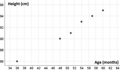
Thus, we have the direction is positive because the pattern in the scatterplot slopes upwards. And the form is linear because there is no strong curvature present in the scatterplot. The strength is strong because the points only deviate very slightly from the general pattern in the points. The unusual points appear to be one outlier because the leftmost point in the scatterplot lies far from the other points in the scatterplot.

(b)

To determine

To find the equation of the least squares regression line using your calculator.

Answer to Problem T3.11SPT

  $\widehat{y}=71.95+0.3833x$ .

Explanation of Solution

Using calculator, press on STAT and then select $1$ : Edit . and then enter the data of sugar in the list $L_1$ and enter the data of calories in the list $L_2$ .

Next, press on STAT select CALC and then select $\text{Linreg}(a+bx)$ . Next we need to finish the command by entering $L_1{L}_2$ .

  $\text{Linreg}(a+bx)L_1{L}_2$

Finally, pressing on ENTER then gives us the following result:

  $\begin{array}{l}y=a+bx\\ a=71.95\\ b=0.3833\\ r^2=0.9888\\ r=0.9944\end{array}$

This then implies the regression line as:

  $\begin{array}{l}\widehat{y}=a+bx\\ \Rightarrow \widehat{y}=71.95+0.3833x\end{array}$

Where x be age and y be height.

(c)

To determine

To calculate and interpret the residual for the point when Sarah was $48$ months old.

Answer to Problem T3.11SPT

Residual is $-0.3484$ .

Explanation of Solution

The regression line is:

  $\widehat{y}=71.95+0.3833x$

Thus, the height of Sarah will be when Sarah was $48$ months old:

  $\begin{array}{l}\widehat{y}=71.95+0.3833x\\ =71.95+0.3833(48)\\ =90.3484\end{array}$

The residual will be as:

  $\begin{array}{l}\text{Residual}=y-\widehat{y}\\ =90-90.3484\\ =-0.3484\end{array}$

This then implies that we overestimated the height of Sarah by $0.3484$ cm, when making a prediction using the regression line.

(d)

To determine

To explain would you be confident using the equation from part (b) to predict Sarah’s height when she was $48$ months old.

Answer to Problem T3.11SPT

No, we are not.

Explanation of Solution

Since there are twelve months in a year then $40$ years corresponds with

  $\begin{array}{l}40\times 12\\ =480\end{array}$

The data contains ages from $36\text{ months to 60}$ months. We then note that $480$ months is not in the range of the ages, which implies that we would not be confident using the equation from part (b) to predict Sarah’s height when Sarah was $48$ months old because we would be using extrapolation.