
Videos
a.
To know that in a random sample of 30 Bounty paper towels and a random sample of 30 generic paper towels, the manufacturer claims that they are the "quicker picker-upper," but are they also the stronger picker-upper? And also to know would it be appropriate to use frequency histograms instead of relative frequency histograms in this setting.
a.
Answer to Problem 76E
Yes, it would be appropriate to use frequency histograms instead of relative frequency histograms in this setting.
Explanation of Solution
Given a random sample of 30 Bounty paper towels and a random sample of 30 generic paper towels and measured their strength when wet. To do this, they uniformly soaked each paper towel with 4 ounces of water, held two opposite edges of the paper towel, and counted how many quarters each paper towel could hold until ripping, alternating brands. The data are displayed in the relative frequency histogram shown below:
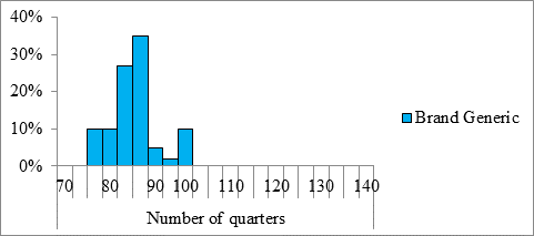
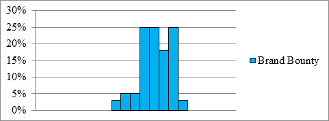
It would be appropriate to use frequency histograms instead of relative frequency histograms, because the two histograms are based on the same number of data values (as there are 30 Bounty paper towels and 30 Generic paper towels in the two samples). Since these two histograms would be based on the same number of data values, we would be able to compare the frequency histograms.
b.
To know that in a random sample of 30 Bounty paper towels and a random sample of 30 generic paper towels, the manufacturer claims that they are the "quicker picker-upper," but are they also the stronger picker-upper? And also to compare the distributions of number of quarters until breaking for the two paper towel brands.
b.
Answer to Problem 76E
The generic distribution is roughly symmetric, while the bounty distribution is skewed to the left.
Neither distribution appears to contain any outliers.
The center of the generic distribution is roughly at 90 quarters, while we expect the center of the bounty distribution to be roughly at 120 quarters.
The spread of the both distributions appears to be roughly the same.
Explanation of Solution
Given a random sample of 30 Bounty paper towels and a random sample of 30 generic paper towels and measured their strength when wet. To do this, they uniformly soaked each paper towel with 4 ounces of water, held two opposite edges of the paper towel, and counted how many quarters each paper towel could hold until ripping, alternating brands. The data are displayed in the relative frequency histogram shown below:
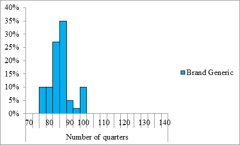
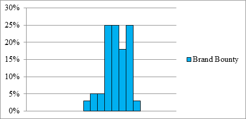
The generic distribution is roughly symmetric, because the highest bars are roughly in the middle of the distribution as shown in the histogram above. The bounty distribution is skewed to the left, because the highest bars are to the right in the histogram above with a tail of smaller bars to the left.
Neither distribution appears to contain any outliers, because there are no gaps in the histograms shown above.
The center of the generic distribution is roughly at 90 quarters, as we expect the center to be roughly at the highest bar in the histogram. Similarly, we expect the center of the bounty distribution to be roughly at 120 quarters.
The spread of the both distributions appears to be roughly the same, because one distribution uses 7 bars and the other distribution uses 8 bars of the same width in the histogram.
Chapter 1 Solutions
EBK PRACTICE OF STAT.F/AP EXAM,UPDATED
Additional Math Textbook Solutions
A First Course in Probability (10th Edition)
Basic Business Statistics, Student Value Edition
Algebra and Trigonometry (6th Edition)
A Problem Solving Approach To Mathematics For Elementary School Teachers (13th Edition)
University Calculus: Early Transcendentals (4th Edition)


- For a binary asymmetric channel with Py|X(0|1) = 0.1 and Py|X(1|0) = 0.2; PX(0) = 0.4 isthe probability of a bit of “0” being transmitted. X is the transmitted digit, and Y is the received digit.a. Find the values of Py(0) and Py(1).b. What is the probability that only 0s will be received for a sequence of 10 digits transmitted?c. What is the probability that 8 1s and 2 0s will be received for the same sequence of 10 digits?d. What is the probability that at least 5 0s will be received for the same sequence of 10 digits?arrow_forwardV2 360 Step down + I₁ = I2 10KVA 120V 10KVA 1₂ = 360-120 or 2nd Ratio's V₂ m 120 Ratio= 360 √2 H I2 I, + I2 120arrow_forwardQ2. [20 points] An amplitude X of a Gaussian signal x(t) has a mean value of 2 and an RMS value of √(10), i.e. square root of 10. Determine the PDF of x(t).arrow_forward
- In a network with 12 links, one of the links has failed. The failed link is randomlylocated. An electrical engineer tests the links one by one until the failed link is found.a. What is the probability that the engineer will find the failed link in the first test?b. What is the probability that the engineer will find the failed link in five tests?Note: You should assume that for Part b, the five tests are done consecutively.arrow_forwardProblem 3. Pricing a multi-stock option the Margrabe formula The purpose of this problem is to price a swap option in a 2-stock model, similarly as what we did in the example in the lectures. We consider a two-dimensional Brownian motion given by W₁ = (W(¹), W(2)) on a probability space (Q, F,P). Two stock prices are modeled by the following equations: dX = dY₁ = X₁ (rdt+ rdt+0₁dW!) (²)), Y₁ (rdt+dW+0zdW!"), with Xo xo and Yo =yo. This corresponds to the multi-stock model studied in class, but with notation (X+, Y₁) instead of (S(1), S(2)). Given the model above, the measure P is already the risk-neutral measure (Both stocks have rate of return r). We write σ = 0₁+0%. We consider a swap option, which gives you the right, at time T, to exchange one share of X for one share of Y. That is, the option has payoff F=(Yr-XT). (a) We first assume that r = 0 (for questions (a)-(f)). Write an explicit expression for the process Xt. Reminder before proceeding to question (b): Girsanov's theorem…arrow_forwardProblem 1. Multi-stock model We consider a 2-stock model similar to the one studied in class. Namely, we consider = S(1) S(2) = S(¹) exp (σ1B(1) + (M1 - 0/1 ) S(²) exp (02B(2) + (H₂- M2 where (B(¹) ) +20 and (B(2) ) +≥o are two Brownian motions, with t≥0 Cov (B(¹), B(2)) = p min{t, s}. " The purpose of this problem is to prove that there indeed exists a 2-dimensional Brownian motion (W+)+20 (W(1), W(2))+20 such that = S(1) S(2) = = S(¹) exp (011W(¹) + (μ₁ - 01/1) t) 롱) S(²) exp (021W (1) + 022W(2) + (112 - 03/01/12) t). where σ11, 21, 22 are constants to be determined (as functions of σ1, σ2, p). Hint: The constants will follow the formulas developed in the lectures. (a) To show existence of (Ŵ+), first write the expression for both W. (¹) and W (2) functions of (B(1), B(²)). as (b) Using the formulas obtained in (a), show that the process (WA) is actually a 2- dimensional standard Brownian motion (i.e. show that each component is normal, with mean 0, variance t, and that their…arrow_forward
- The scores of 8 students on the midterm exam and final exam were as follows. Student Midterm Final Anderson 98 89 Bailey 88 74 Cruz 87 97 DeSana 85 79 Erickson 85 94 Francis 83 71 Gray 74 98 Harris 70 91 Find the value of the (Spearman's) rank correlation coefficient test statistic that would be used to test the claim of no correlation between midterm score and final exam score. Round your answer to 3 places after the decimal point, if necessary. Test statistic: rs =arrow_forwardBusiness discussarrow_forwardBusiness discussarrow_forward
 MATLAB: An Introduction with ApplicationsStatisticsISBN:9781119256830Author:Amos GilatPublisher:John Wiley & Sons Inc
 Probability and Statistics for Engineering and th...StatisticsISBN:9781305251809Author:Jay L. DevorePublisher:Cengage Learning
 Statistics for The Behavioral Sciences (MindTap C...StatisticsISBN:9781305504912Author:Frederick J Gravetter, Larry B. WallnauPublisher:Cengage Learning
 Elementary Statistics: Picturing the World (7th E...StatisticsISBN:9780134683416Author:Ron Larson, Betsy FarberPublisher:PEARSON
 The Basic Practice of StatisticsStatisticsISBN:9781319042578Author:David S. Moore, William I. Notz, Michael A. FlignerPublisher:W. H. Freeman
 Introduction to the Practice of StatisticsStatisticsISBN:9781319013387Author:David S. Moore, George P. McCabe, Bruce A. CraigPublisher:W. H. Freeman