
Videos
a.
To find what proportion of the water python eggs that hatched were randomly assigned to hot water.
a.
Answer to Problem 32E
About 0.5814 of the hatched eggs were assigned to hot water.
Explanation of Solution
Given:
| Water temperature | |||||
| Cold | Neutral | Hot | Total | ||
| Hatched? | Yes | 16 | 38 | 75 | 129 |
| No | 11 | 18 | 29 | 58 | |
| Total | 27 | 56 | 104 | 187 | |
Calculation:
The study includes 187 eggs (as the value 187 is mentioned in the bottom right corner of the given table).
| Water temperature | |||||
| Cold | Neutral | Hot | Total | ||
| Hatched? | Yes | 16 | 38 | 75 | 129 |
| No | 11 | 18 | 29 | 58 | |
| Total | 27 | 56 | 104 | 187 | |
We note that 129 of the 187 eggs hatched (as 129 is mentioned in the row "Yes" and in the column "Total" of the given table).
Moreover, we also note that 75 of the 129 hatched eggs were assigned to hot water (as 75 is mentioned in the row "Yes" and in the column "Hot" of the given table).
Thus about 0.5814 of the hatched eggs were assigned to hot water.
b.
To find what percentage of the water python eggs that were randomly assigned to hot water have hatched.
b.
Answer to Problem 32E
About 72.12% of the eggs assigned to hot water have hatched.
Explanation of Solution
Given:
Researchers randomly assigned newly laid water python eggs to one of three water temperatures: hot, neutral, or cold. Hot duplicates the extra warmth provided by the mother python, and cold duplicates the absence of the mother. The below two-way table summarizes the data on whether or not the eggs hatched.
| Water temperature | |||||
| Cold | Neutral | Hot | Total | ||
| Hatched? | Yes | 16 | 38 | 75 | 129 |
| No | 11 | 18 | 29 | 58 | |
| Total | 27 | 56 | 104 | 187 | |
Calculation:
The study includes 187 eggs (as the value 187 is mentioned in the bottom right corner of the given table).
| Water temperature | |||||
| Cold | Neutral | Hot | Total | ||
| Hatched? | Yes | 16 | 38 | 75 | 129 |
| No | 11 | 18 | 29 | 58 | |
| Total | 27 | 56 | 104 | 187 | |
We note that 104 of the 187 eggs were assigned to hot water (as 104is mentioned in the row "Total" and in the column "Hot" of the given table).
Moreover, we also note that 75 of the 104eggs assigned to hot water have hatched (as 75 is mentioned in the row "Yes" and in the column "Hot" of the given table).
Thus about 72.12% of the eggs assigned to hot water have hatched.
c.
To describe the segmented bar graph that displays the distribution of hatching status by water temperature and what it actually reveals about the association between these two variables for the python eggs in this experiment.
c.
Answer to Problem 32E
Eggs appears to be more likely to hatch as the temperature increases. We note that for each temperature, the majority of the eggs latch.
Explanation of Solution
The below segmented bar graph displays the information about the distribution of hatching status (%) by water temperature:
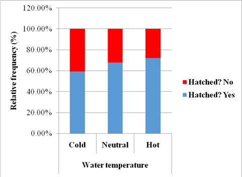
We note that eggs appears to be more likely to hatch as the temperature increases, because when comparing the blue parts of the bars of the segmented bar graph, we note that the blue section is smallest for "Low" and largest for "High" temperature.
We note that for each temperature, the majority of the eggs hatch, because the blue section of each bar is larger than the red section of the bar.
Chapter 1 Solutions
EBK PRACTICE OF STAT.F/AP EXAM,UPDATED
Additional Math Textbook Solutions
Thinking Mathematically (6th Edition)
Pre-Algebra Student Edition
Algebra and Trigonometry (6th Edition)
Elementary Statistics (13th Edition)
College Algebra with Modeling & Visualization (5th Edition)
University Calculus: Early Transcendentals (4th Edition)


- Questions An insurance company's cumulative incurred claims for the last 5 accident years are given in the following table: Development Year Accident Year 0 2018 1 2 3 4 245 267 274 289 292 2019 255 276 288 294 2020 265 283 292 2021 263 278 2022 271 It can be assumed that claims are fully run off after 4 years. The premiums received for each year are: Accident Year Premium 2018 306 2019 312 2020 318 2021 326 2022 330 You do not need to make any allowance for inflation. 1. (a) Calculate the reserve at the end of 2022 using the basic chain ladder method. (b) Calculate the reserve at the end of 2022 using the Bornhuetter-Ferguson method. 2. Comment on the differences in the reserves produced by the methods in Part 1.arrow_forwardTo help consumers in purchasing a laptop computer, Consumer Reports calculates an overall test score for each computer tested based upon rating factors such as ergonomics, portability, performance, display, and battery life. Higher overall scores indicate better test results. The following data show the average retail price and the overall score for ten 13-inch models (Consumer Reports website, October 25, 2012). Brand & Model Price ($) Overall Score Samsung Ultrabook NP900X3C-A01US 1250 83 Apple MacBook Air MC965LL/A 1300 83 Apple MacBook Air MD231LL/A 1200 82 HP ENVY 13-2050nr Spectre XT 950 79 Sony VAIO SVS13112FXB 800 77 Acer Aspire S5-391-9880 Ultrabook 1200 74 Apple MacBook Pro MD101LL/A 1200 74 Apple MacBook Pro MD313LL/A 1000 73 Dell Inspiron I13Z-6591SLV 700 67 Samsung NP535U3C-A01US 600 63 a. Select a scatter diagram with price as the independent variable. b. What does the scatter diagram developed in part (a) indicate about the relationship…arrow_forwardTo the Internal Revenue Service, the reasonableness of total itemized deductions depends on the taxpayer’s adjusted gross income. Large deductions, which include charity and medical deductions, are more reasonable for taxpayers with large adjusted gross incomes. If a taxpayer claims larger than average itemized deductions for a given level of income, the chances of an IRS audit are increased. Data (in thousands of dollars) on adjusted gross income and the average or reasonable amount of itemized deductions follow. Adjusted Gross Income ($1000s) Reasonable Amount ofItemized Deductions ($1000s) 22 9.6 27 9.6 32 10.1 48 11.1 65 13.5 85 17.7 120 25.5 Compute b1 and b0 (to 4 decimals).b1 b0 Complete the estimated regression equation (to 2 decimals). = + x Predict a reasonable level of total itemized deductions for a taxpayer with an adjusted gross income of $52.5 thousand (to 2 decimals). thousand dollarsWhat is the value, in dollars, of…arrow_forward
- K The mean height of women in a country (ages 20-29) is 63.7 inches. A random sample of 65 women in this age group is selected. What is the probability that the mean height for the sample is greater than 64 inches? Assume σ = 2.68. The probability that the mean height for the sample is greater than 64 inches is (Round to four decimal places as needed.)arrow_forwardIn a survey of a group of men, the heights in the 20-29 age group were normally distributed, with a mean of 69.6 inches and a standard deviation of 4.0 inches. A study participant is randomly selected. Complete parts (a) through (d) below. (a) Find the probability that a study participant has a height that is less than 68 inches. The probability that the study participant selected at random is less than 68 inches tall is 0.4. (Round to four decimal places as needed.) 20 2arrow_forwardPEER REPLY 1: Choose a classmate's Main Post and review their decision making process. 1. Choose a risk level for each of the states of nature (assign a probability value to each). 2. Explain why each risk level is chosen. 3. Which alternative do you believe would be the best based on the maximum EMV? 4. Do you feel determining the expected value with perfect information (EVWPI) is worthwhile in this situation? Why or why not?arrow_forward
- Questions An insurance company's cumulative incurred claims for the last 5 accident years are given in the following table: Development Year Accident Year 0 2018 1 2 3 4 245 267 274 289 292 2019 255 276 288 294 2020 265 283 292 2021 263 278 2022 271 It can be assumed that claims are fully run off after 4 years. The premiums received for each year are: Accident Year Premium 2018 306 2019 312 2020 318 2021 326 2022 330 You do not need to make any allowance for inflation. 1. (a) Calculate the reserve at the end of 2022 using the basic chain ladder method. (b) Calculate the reserve at the end of 2022 using the Bornhuetter-Ferguson method. 2. Comment on the differences in the reserves produced by the methods in Part 1.arrow_forwardYou are provided with data that includes all 50 states of the United States. Your task is to draw a sample of: o 20 States using Random Sampling (2 points: 1 for random number generation; 1 for random sample) o 10 States using Systematic Sampling (4 points: 1 for random numbers generation; 1 for random sample different from the previous answer; 1 for correct K value calculation table; 1 for correct sample drawn by using systematic sampling) (For systematic sampling, do not use the original data directly. Instead, first randomize the data, and then use the randomized dataset to draw your sample. Furthermore, do not use the random list previously generated, instead, generate a new random sample for this part. For more details, please see the snapshot provided at the end.) Upload a Microsoft Excel file with two separate sheets. One sheet provides random sampling while the other provides systematic sampling. Excel snapshots that can help you in organizing columns are provided on the next…arrow_forwardThe population mean and standard deviation are given below. Find the required probability and determine whether the given sample mean would be considered unusual. For a sample of n = 65, find the probability of a sample mean being greater than 225 if μ = 224 and σ = 3.5. For a sample of n = 65, the probability of a sample mean being greater than 225 if μ=224 and σ = 3.5 is 0.0102 (Round to four decimal places as needed.)arrow_forward
- ***Please do not just simply copy and paste the other solution for this problem posted on bartleby as that solution does not have all of the parts completed for this problem. Please answer this I will leave a like on the problem. The data needed to answer this question is given in the following link (file is on view only so if you would like to make a copy to make it easier for yourself feel free to do so) https://docs.google.com/spreadsheets/d/1aV5rsxdNjHnkeTkm5VqHzBXZgW-Ptbs3vqwk0SYiQPo/edit?usp=sharingarrow_forwardThe data needed to answer this question is given in the following link (file is on view only so if you would like to make a copy to make it easier for yourself feel free to do so) https://docs.google.com/spreadsheets/d/1aV5rsxdNjHnkeTkm5VqHzBXZgW-Ptbs3vqwk0SYiQPo/edit?usp=sharingarrow_forwardThe following relates to Problems 4 and 5. Christchurch, New Zealand experienced a major earthquake on February 22, 2011. It destroyed 100,000 homes. Data were collected on a sample of 300 damaged homes. These data are saved in the file called CIEG315 Homework 4 data.xlsx, which is available on Canvas under Files. A subset of the data is shown in the accompanying table. Two of the variables are qualitative in nature: Wall construction and roof construction. Two of the variables are quantitative: (1) Peak ground acceleration (PGA), a measure of the intensity of ground shaking that the home experienced in the earthquake (in units of acceleration of gravity, g); (2) Damage, which indicates the amount of damage experienced in the earthquake in New Zealand dollars; and (3) Building value, the pre-earthquake value of the home in New Zealand dollars. PGA (g) Damage (NZ$) Building Value (NZ$) Wall Construction Roof Construction Property ID 1 0.645 2 0.101 141,416 2,826 253,000 B 305,000 B T 3…arrow_forward
 MATLAB: An Introduction with ApplicationsStatisticsISBN:9781119256830Author:Amos GilatPublisher:John Wiley & Sons Inc
 Probability and Statistics for Engineering and th...StatisticsISBN:9781305251809Author:Jay L. DevorePublisher:Cengage Learning
 Statistics for The Behavioral Sciences (MindTap C...StatisticsISBN:9781305504912Author:Frederick J Gravetter, Larry B. WallnauPublisher:Cengage Learning
 Elementary Statistics: Picturing the World (7th E...StatisticsISBN:9780134683416Author:Ron Larson, Betsy FarberPublisher:PEARSON
 The Basic Practice of StatisticsStatisticsISBN:9781319042578Author:David S. Moore, William I. Notz, Michael A. FlignerPublisher:W. H. Freeman
 Introduction to the Practice of StatisticsStatisticsISBN:9781319013387Author:David S. Moore, George P. McCabe, Bruce A. CraigPublisher:W. H. Freeman