
Concept explainers
Videos
a.
To describe the overall shape of the distribution of monthly returns for the U.S. stock market over a 273-month period.
a.
Answer to Problem 71E
The distribution is skewed to the left and the distribution appears to contain 3 outliers with 2 gaps.
Explanation of Solution
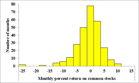
The figure below shows a histogram of the distribution of monthly returns for the U.S. stock market over a 273-month period:

The distribution is skewed to the left, because the highest bars are to the right in the histogram with a tail of smaller bars to the left.
The distribution appears to contain 3 outliers, because there are two bars (one with frequency 2 and the other with frequency 1) which are separated by a gap from the other bars of the histogram.
The gaps are roughly at -20 and -13, while there are two potential outliers between -25 and -22.5, with one other potential outlier between -17.5 and -15.
b.
To determine the approximate center of this distribution of monthly returns for the U.S. stock market over a 273-month period.
b.
Answer to Problem 71E
The center of this distribution to be between 0% and 2.5%.
Explanation of Solution
The figure below shows a histogram of the distribution of monthly returns for the U.S. stock market over a 273-month period:
We expect the center of the distribution to be roughly at the highest bar in the histogram.
The highest bar has monthly percent returns between 0% and 2.5%, thus we then estimate the center of this distribution to be between 0% and 2.5%.
c.
To determine why we cannot find the exact value for the minimum return and between what two values does it lie.
c.
Answer to Problem 71E
We cannot determine the exact value of the minimum return, because we have not been given its exact value and we only know a
The minimum return is between -25% and -22.5%.
Explanation of Solution
The figure below shows a histogram of the distribution of monthly returns for the U.S. stock market over a 273-month period:

The minimum return is represented by the left most bar in the histogram.
However, we cannot determine the exact value of the minimum return, because we have not been given its exact value and we only know a range of possible values for the minimum return by the corresponding bar in the histogram.
We note that the leftmost bar in the histogram takes on monthly percent returns on common stocks between -25% and -22.5%, which then implies that the minimum return is between -25% and -22.5%.
d.
To determine about what percent of all months had returns less than 0 for the U.S. stock market over a 273-month period.
d.
Answer to Problem 71E
Approximately, 37.36% of the months has returns less than 0.
Explanation of Solution
The figure below shows a histogram of the distribution of monthly returns for the U.S. stock market over a 273-month period:

Let us first estimate the frequency of corresponding to the interval of each bar, which is given by the height of the bars.
| Interval | Frequency |
| -25 < -22.5 | 2 |
| -22.5 < -20 | 0 |
| -20 < -17.5 | 0 |
| -17.5 < -15 | 1 |
| -15 < -12.5 | 0 |
| -12.5 < -10 | 4 |
| -10 < -7.5 | 6 |
| -7.5 < -5 | 11 |
| -5 < -2.5 | 28 |
| -2.5 < 0 | 50 |
| 0 < 2.5 | 78 |
| 2.5 < 5 | 58 |
| 5 < 7.5 | 24 |
| 7.5 < 10 | 8 |
| 10 < 12.5 | 3 |
Let us next add the frequencies of all intervals with negative returns.

Thus we then note that 102 of the 273 months in the sample have a return less than 0.
This then implies that approximately 37.36% of the months has returns less than 0.
Chapter 1 Solutions
EBK PRACTICE OF STAT.F/AP EXAM,UPDATED
Additional Math Textbook Solutions
Calculus: Early Transcendentals (2nd Edition)
Calculus for Business, Economics, Life Sciences, and Social Sciences (14th Edition)
Calculus: Early Transcendentals (2nd Edition)
A Problem Solving Approach To Mathematics For Elementary School Teachers (13th Edition)


- For a binary asymmetric channel with Py|X(0|1) = 0.1 and Py|X(1|0) = 0.2; PX(0) = 0.4 isthe probability of a bit of “0” being transmitted. X is the transmitted digit, and Y is the received digit.a. Find the values of Py(0) and Py(1).b. What is the probability that only 0s will be received for a sequence of 10 digits transmitted?c. What is the probability that 8 1s and 2 0s will be received for the same sequence of 10 digits?d. What is the probability that at least 5 0s will be received for the same sequence of 10 digits?arrow_forwardV2 360 Step down + I₁ = I2 10KVA 120V 10KVA 1₂ = 360-120 or 2nd Ratio's V₂ m 120 Ratio= 360 √2 H I2 I, + I2 120arrow_forwardQ2. [20 points] An amplitude X of a Gaussian signal x(t) has a mean value of 2 and an RMS value of √(10), i.e. square root of 10. Determine the PDF of x(t).arrow_forward
- In a network with 12 links, one of the links has failed. The failed link is randomlylocated. An electrical engineer tests the links one by one until the failed link is found.a. What is the probability that the engineer will find the failed link in the first test?b. What is the probability that the engineer will find the failed link in five tests?Note: You should assume that for Part b, the five tests are done consecutively.arrow_forwardProblem 3. Pricing a multi-stock option the Margrabe formula The purpose of this problem is to price a swap option in a 2-stock model, similarly as what we did in the example in the lectures. We consider a two-dimensional Brownian motion given by W₁ = (W(¹), W(2)) on a probability space (Q, F,P). Two stock prices are modeled by the following equations: dX = dY₁ = X₁ (rdt+ rdt+0₁dW!) (²)), Y₁ (rdt+dW+0zdW!"), with Xo xo and Yo =yo. This corresponds to the multi-stock model studied in class, but with notation (X+, Y₁) instead of (S(1), S(2)). Given the model above, the measure P is already the risk-neutral measure (Both stocks have rate of return r). We write σ = 0₁+0%. We consider a swap option, which gives you the right, at time T, to exchange one share of X for one share of Y. That is, the option has payoff F=(Yr-XT). (a) We first assume that r = 0 (for questions (a)-(f)). Write an explicit expression for the process Xt. Reminder before proceeding to question (b): Girsanov's theorem…arrow_forwardProblem 1. Multi-stock model We consider a 2-stock model similar to the one studied in class. Namely, we consider = S(1) S(2) = S(¹) exp (σ1B(1) + (M1 - 0/1 ) S(²) exp (02B(2) + (H₂- M2 where (B(¹) ) +20 and (B(2) ) +≥o are two Brownian motions, with t≥0 Cov (B(¹), B(2)) = p min{t, s}. " The purpose of this problem is to prove that there indeed exists a 2-dimensional Brownian motion (W+)+20 (W(1), W(2))+20 such that = S(1) S(2) = = S(¹) exp (011W(¹) + (μ₁ - 01/1) t) 롱) S(²) exp (021W (1) + 022W(2) + (112 - 03/01/12) t). where σ11, 21, 22 are constants to be determined (as functions of σ1, σ2, p). Hint: The constants will follow the formulas developed in the lectures. (a) To show existence of (Ŵ+), first write the expression for both W. (¹) and W (2) functions of (B(1), B(²)). as (b) Using the formulas obtained in (a), show that the process (WA) is actually a 2- dimensional standard Brownian motion (i.e. show that each component is normal, with mean 0, variance t, and that their…arrow_forward
- The scores of 8 students on the midterm exam and final exam were as follows. Student Midterm Final Anderson 98 89 Bailey 88 74 Cruz 87 97 DeSana 85 79 Erickson 85 94 Francis 83 71 Gray 74 98 Harris 70 91 Find the value of the (Spearman's) rank correlation coefficient test statistic that would be used to test the claim of no correlation between midterm score and final exam score. Round your answer to 3 places after the decimal point, if necessary. Test statistic: rs =arrow_forwardBusiness discussarrow_forwardBusiness discussarrow_forward
 MATLAB: An Introduction with ApplicationsStatisticsISBN:9781119256830Author:Amos GilatPublisher:John Wiley & Sons Inc
 Probability and Statistics for Engineering and th...StatisticsISBN:9781305251809Author:Jay L. DevorePublisher:Cengage Learning
 Statistics for The Behavioral Sciences (MindTap C...StatisticsISBN:9781305504912Author:Frederick J Gravetter, Larry B. WallnauPublisher:Cengage Learning
 Elementary Statistics: Picturing the World (7th E...StatisticsISBN:9780134683416Author:Ron Larson, Betsy FarberPublisher:PEARSON
 The Basic Practice of StatisticsStatisticsISBN:9781319042578Author:David S. Moore, William I. Notz, Michael A. FlignerPublisher:W. H. Freeman
 Introduction to the Practice of StatisticsStatisticsISBN:9781319013387Author:David S. Moore, George P. McCabe, Bruce A. CraigPublisher:W. H. Freeman