
Concept explainers
a)
To determine: The mean of each sample.
a)
Answer to Problem 20P
Explanation of Solution
Given information:
| Sample | |||
| 1 | 2 | 3 | 4 |
| 4.5 | 4.6 | 4.5 | 4.7 |
| 4.2 | 4.5 | 4.6 | 4.6 |
| 4.2 | 4.4 | 4.4 | 4.8 |
| 4.3 | 4.7 | 4.4 | 4.5 |
| 4.3 | 4.3 | 4.6 | 4.9 |
Calculation of mean of each sample:
| Sample | ||||
| Sl. No. | 1 | 2 | 3 | 4 |
| 1 | 4.5 | 4.6 | 4.5 | 4.7 |
| 2 | 4.2 | 4.5 | 4.6 | 4.6 |
| 3 | 4.2 | 4.4 | 4.4 | 4.8 |
| 4 | 4.3 | 4.7 | 4.4 | 4.5 |
| 5 | 4.3 | 4.3 | 4.6 | 4.9 |
| Mean | 4.3 | 4.5 | 4.5 | 4.7 |
Table 1
Excel Worksheet:
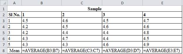
Sample 1:
The mean is calculated by adding each sample points. Adding the points 4.5, 4.2, 4.2, 4.3 and 4.3 and dividing by 5 gives mean of 4.3. The same process is followed for finding mean for other samples.
Hence, the mean of each sample is shown in Table 1
b)
To determine: The mean and standard deviation when the process parameters are unknown.
b)
Answer to Problem 20P
Explanation of Solution
Given information:
| Sample | |||
| 1 | 2 | 3 | 4 |
| 4.5 | 4.6 | 4.5 | 4.7 |
| 4.2 | 4.5 | 4.6 | 4.6 |
| 4.2 | 4.4 | 4.4 | 4.8 |
| 4.3 | 4.7 | 4.4 | 4.5 |
| 4.3 | 4.3 | 4.6 | 4.9 |
Calculation of mean and standard deviation:
Table 1 provides the mean for each sample points.
The mean is calculated by adding each mean of the samples. Adding the points 4.3, 4.5, 4.5 and 4.7 and dividing by 4 gives mean of 4.5.
The standard deviation is calculated using the above formula and substituting the values of mean in the above formula and the resultant of 0.192 is obtained.
Hence, the mean and standard deviation when the process parameters are unknown are 4.5 and 0.192.
c)
To determine: The mean and standard deviation of the sampling distribution.
c)
Answer to Problem 20P
Explanation of Solution
Given information:
| Sample | |||
| 1 | 2 | 3 | 4 |
| 4.5 | 4.6 | 4.5 | 4.7 |
| 4.2 | 4.5 | 4.6 | 4.6 |
| 4.2 | 4.4 | 4.4 | 4.8 |
| 4.3 | 4.7 | 4.4 | 4.5 |
| 4.3 | 4.3 | 4.6 | 4.9 |
Calculation of mean and standard deviation of the sampling distribution:
From calculation of mean of each samples, the mean for sampling distribution can be computed, the mean for sampling distribution is 4.5 (refer equation (1)).
The standard deviation of the sampling distribution is calculated by dividing 0.192 with the square root of 5 which gives the resultant as 0.086.
Hence, the mean and standard deviation of the sampling distribution is 4.5 and 0.086 respectively.
d)
To determine: The three-sigma control limit for the process and alpha risk provided by them.
d)
Answer to Problem 20P
Explanation of Solution
Given information:
| Sample | |||
| 1 | 2 | 3 | 4 |
| 4.5 | 4.6 | 4.5 | 4.7 |
| 4.2 | 4.5 | 4.6 | 4.6 |
| 4.2 | 4.4 | 4.4 | 4.8 |
| 4.3 | 4.7 | 4.4 | 4.5 |
| 4.3 | 4.3 | 4.6 | 4.9 |
Calculation of three-sigma control limit for the process:
The three-sigma control limits for the process is calculated by multiplying 3.00 with 0.086 (refer equation (2)) and the resultant is added with 4.5 to get an upper control limit which is 4.758 and subtracted to get lower control limit which is 4.242. Using z-factor table z = +3.00 corresponds to 0.4987.
The alpha risk is calculated to be as 0.0026.
Hence, the three-sigma control limits for the process are 4.758 and 4.242.
e)
To determine: The alpha risk for control limits of 4.14 and 4.86.
e)
Answer to Problem 20P
Explanation of Solution
Given information:
| Sample | |||
| 1 | 2 | 3 | 4 |
| 4.5 | 4.6 | 4.5 | 4.7 |
| 4.2 | 4.5 | 4.6 | 4.6 |
| 4.2 | 4.4 | 4.4 | 4.8 |
| 4.3 | 4.7 | 4.4 | 4.5 |
| 4.3 | 4.3 | 4.6 | 4.9 |
Formula:
Calculation alpha risk for control limits of 4.14 and 4.86:
The alpha risk is calculated by dividing the difference of 4.86 and 4.5 with 0.086 which gives +4.19 which is the risk is close to zero.
Hence, the alpha risk for control limits of 4.14 and 4.86 is +4.1
f)
To determine: Whether any of the sample means are beyond the control limits.
f)
Answer to Problem 20P
Explanation of Solution
Given information:
| Sample | |||
| 1 | 2 | 3 | 4 |
| 4.5 | 4.6 | 4.5 | 4.7 |
| 4.2 | 4.5 | 4.6 | 4.6 |
| 4.2 | 4.4 | 4.4 | 4.8 |
| 4.3 | 4.7 | 4.4 | 4.5 |
| 4.3 | 4.3 | 4.6 | 4.9 |
Determination of whether any of the sample means are beyond the control limits:
Table 1 provides the sample means for each sample. From observation, it can be found that each sample mean are within the control limit of 4.14 and 4.86. Therefore, each sample means lies within the control limits of 4.14 and 4.86.
Hence, there are no sample means which lies beyond the control limits.
g)
To determine: Whether any of the samples are beyond the control limits.
g)
Answer to Problem 20P
Explanation of Solution
Given information:
| SAMPLE | |||
| 1 | 2 | 3 | 4 |
| 4.5 | 4.6 | 4.5 | 4.7 |
| 4.2 | 4.5 | 4.6 | 4.6 |
| 4.2 | 4.4 | 4.4 | 4.8 |
| 4.3 | 4.7 | 4.4 | 4.5 |
| 4.3 | 4.3 | 4.6 | 4.9 |
Formula:
Mean Chart:
Range Chart:
Calculation of upper and lower control limits:
| SAMPLE | ||||
| 1 | 2 | 3 | 4 | |
| 4.5 | 4.6 | 4.5 | 4.7 | |
| 4.2 | 4.5 | 4.6 | 4.6 | |
| 4.2 | 4.4 | 4.4 | 4.8 | |
| 4.3 | 4.7 | 4.4 | 4.5 | |
| 4.3 | 4.3 | 4.6 | 4.9 | |
| Mean | 4.3 | 4.5 | 4.5 | 4.7 |
| Range | .3 | .4 | .2 | .4 |
From factors of three-sigma chart, A2 = 0.58; D3 = 0; D4 = 2.11.
Mean control chart:
Upper control limit:
The Upper control limit is calculated by adding the product of 0.58 and 0.325 with 4.5 which yields 4.689.
Lower control limit:
The Lower control limit is calculated by subtracting the product of 0.58 and 0.325 with 4.5 which yields 4.311.
The UCL and LCL for mean charts are 4.686 and 4.311. (4)
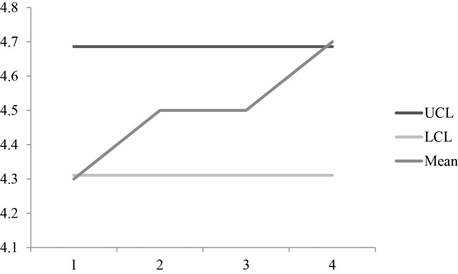
A graph is plotted using the UCL and LCL and mean values which shows the points are within the control limits.
Range control chart:
Upper control limit:
The Upper control limit is calculated by multiplying 2.11 with 0.325 which yields 0.686.
Lower control limit:
The lower control limit is calculated by multiplying 0 with 0.325 which yields 0.0.
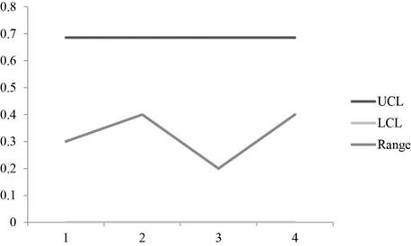
A graph is plotted using the UCL, LCL and Range values which shows that the points are within the control region.
Hence, all points are within control limits.
h)
To explain: The reason for variations in control limits.
h)
Answer to Problem 20P
Explanation of Solution
Reason for variations in control limits:
The control limits vary because in equation (3) and (4) because of the use of different measure for dispersion to measure the standard deviation and range.
Hence, the difference arises due to the use of different measures for dispersion to the measure the standard deviation and range.
i)
To determine: The control limits for the process and whether the process will be in control.
i)
Answer to Problem 20P
Explanation of Solution
Given information:
Determination of control limits of the process:
Sample mean is given in Table 1.
To calculate the control limits 0.18 is divided by root of 5 and is multiplied by 3 and the resultant is added to 4.4 to give UCL which is 4.641 and subtracted from 4.4 to get the LCL which is 4.159.
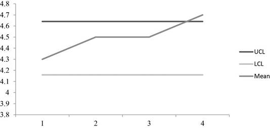
The graph shows that the some of the points are above the control limits which make the process to be out of control.
Hence, the process is out of control with UCL=4.641 and LCL=4.159.
Want to see more full solutions like this?
Chapter 10 Solutions
Operations Management (Comp. Instructor's Edition)


- Examine the conflicts between improving customer service levels and controlling costs in sales. Strategies to Balance Both customer service levels and controlling costs in sales 1.Outsourcing and workforce optimization 2. AI-driven customer supportarrow_forwardhow can you gain trust in a negotiation setting?arrow_forward✓ Custom $€ .0 .on File Home Insert Share Page Layout Formulas Data Review View Help Draw Arial 10 B B14 ✓ X✓ fx 1400 > 甘く 曲 > 冠 > Comments Editing ✓ . . . P Q R S T 3 A Production cost ($/unit) B с D E F G H J K L M N $74.00 4 Inventory holding cost ($/unit) $1.50 5 Lost sales cost ($/unit) $82.00 6 Overtime cost ($/unit) $6.80 7 Undertime cost ($/unit) $3.20 8 Rate change cost ($/unit) $5.00 9 Normal production rate (units) 2,000 10 Ending inventory (previous Dec.) 800 11 Cumulative 12 13 Month Demand Cumulative Demand Product Production Availability Ending Inventory Lost Cumulative Cumulative Product Sales 14 January 1,400 1,475 15 FUERANZ222222223323333BRUINE 14 February 1,000 2,275 Month January February Demand Demand Production Availability Ending Inventory Lost Sales 1,400 #N/A 1,475 #N/A #N/A #N/A 1,000 #N/A 2,275 #N/A #N/A #N/A 16 March 1,800 2,275 March 1,800 #N/A 2,275 #N/A #N/A #N/A 17 April 2,700 2,275 April 2,700 #N/A 2,275 #N/A #N/A #N/A 18 May 3,000 2,275 May 3,000 #N/A…arrow_forward
 Practical Management ScienceOperations ManagementISBN:9781337406659Author:WINSTON, Wayne L.Publisher:Cengage,