
(a)
Interpretation:
The liquidus temperature for
Concept Introduction:
On the temperature-composition graph of analloy, the curve above which the alloy exist in the liquid phase is the liquidus curve. The temperature at this curve is maximum known as liquidus temperature at which the crystals in the alloy can coexist with its melt in the
Answer to Problem 10.75P
Liquidus temperature,
Explanation of Solution
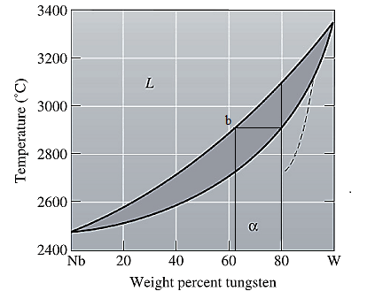
The equilibrium phase diagram for the Nb-W system is shown below as:

A straight line from
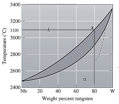
Liquidus temperature
(b)
Interpretation:
The solidus temperature for
Concept Introduction:
Solidus curve is the locus of the temperature on the temperature composition graph of analloy, beyond which the alloy is completely in solid phase. The temperature at this curve is minimum known as solidus temperature at which the crystals in the alloy can coexist with its melt in the thermodynamic equilibrium.
Answer to Problem 10.75P
Solidus temperature,
Explanation of Solution
The equilibrium phase diagram for the Nb-W system is shown below as:

A straight line from
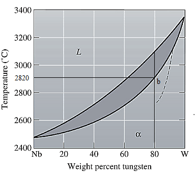
Solidus temperature
(c)
Interpretation:
The freezing range for
Concept Introduction:
Freezing range for analloy is the difference of the liquidus and the solidus temperature of analloy. In this range, the alloy melt starts to crystallize at liquidus temperature and solidifies when reaches solidus temperature.
Answer to Problem 10.75P
Freezing range,
Explanation of Solution
From part (a) and (b), the liquidus and solidus temperature for the given alloy is determined as:
The freezing range (FR) for this alloy composition will be:
(d)
Interpretation:
The composition of the first solid that is formed when
Concept Introduction:
On the temperature-composition graph of analloy, the curve above which the alloy exist in the liquid phase is the liquidus curve. The temperature at this curve is maximum known as liquidus temperature at which the crystals in the alloy can coexist with its melt in the thermodynamic equilibrium.
Answer to Problem 10.75P
The composition of the first solid formed is
Explanation of Solution
The equilibrium phase diagram for the Nb-W system is shown below as:

A straight line from
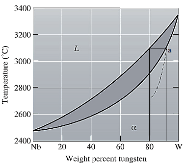
Point 'a' represents the composition of the first solid which is formed when
(e)
Interpretation:
The composition of the last liquid which is solidified when
Concept Introduction:
On the temperature-composition graph of analloy, the curve above which the alloy exist in the liquid phase is the liquidus curve. The temperature at this curve is maximum known as liquidus temperature at which the crystals in the alloy can coexist with its melt in the thermodynamic equilibrium.
Solidus curve is the locus of the temperature on the temperature composition graph of analloy, beyond which the alloy is completely in solid phase.
Between the solidus and liquidus curve, the alloy exits in a slurry form in which there is both crystals as well as alloy melt.
Solidus temperature is always less than or equal to the liquidus temperature.
Answer to Problem 10.75P
The composition of the last liquid solidified is
Explanation of Solution
The equilibrium phase diagram for the Nb-W system is shown below as:
A straight line from
Point 'b' represents the composition of the last liquid which solidify when
(f)
Interpretation:
The phases present, their compositions and their amounts for
Concept Introduction:
On the temperature-composition graph of analloy, the curve above which the alloy exist in the liquid phase is the liquidus curve. The temperature at this curve is the maximum temperature at which the crystals in the alloy can coexist with its melt in the thermodynamic equilibrium.
Solidus curve is the locus of the temperature on the temperature composition graph of analloy, beyond which the alloy is completely in solid phase.
Between the solidus and liquidus curve, the alloy exits in a slurry form in which there is both crystals as well as alloy melt.
Solidus temperature is always less than or equal to the liquidus temperature.
Amount of each phase in wt% is calculated using lever rule. At a particular temperature and alloy composition, a tie line is drawn on the phase diagram of the alloy between the solidus and liquidus curve. Then the portion of the lever opposite to the phase whose amount is to be calculated is considered in the formula used as:
Answer to Problem 10.75P
Both solid as well as liquid phases are present at the given conditions.
Composition of the liquid phase present is
Composition of the solid phase present is
Amount of the liquid phase is
Amount of the solid phase is
Explanation of Solution
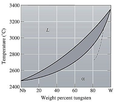
The equilibrium phase diagram for the Nb-W system is shown below as:

Now, draw a straight line from
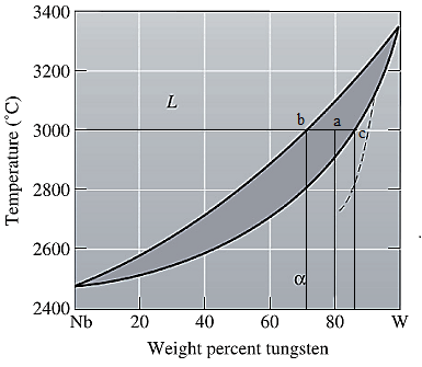
Both the phases, solid and liquid are present at this condition. Point 'b' represents the liquid phase composition in wt% and point 'c' represents the solid phase composition in wt%. From the above phase diagram:
To calculate amount of liquid phase, lever 'ac' will be used and to calculate amount of solid phase, lever 'ba' will be used. Use equation (1) to calculate the amount of each phase as:
(g)
Interpretation:
The phases present, their compositions and their amounts for
Concept Introduction:
On the temperature-composition graph of an alloy, the curve above which the alloy exists in the liquid phase is the liquidus curve. The temperature at this curve is the maximum temperature at which the crystals in the alloy can coexist with its melt in the thermodynamic equilibrium.
Solidus curve is the locus of the temperature on the temperature composition graph of analloy, beyond which the alloy is completely in solid phase.
Between the solidus and liquidus curve, the alloy exits in a slurry form in which there is both crystals as well as alloy melt.
Solidus temperature is always less than or equal to the liquidus temperature.
Amount of each phase in wt% is calculated using lever rule. At a particular temperature and alloy composition, a tie line is drawn on the phase diagram of the alloy between the solidus and liquidus curve. Then the portion of the lever opposite to the phase whose amount is to be calculated is considered in the formula used as:
Answer to Problem 10.75P
Explanation of Solution
The equilibrium phase diagram for the Nb-W system is shown below as:

Now, draw a straight line from
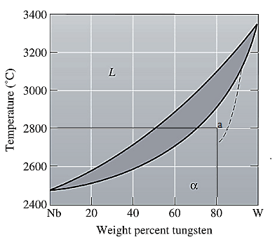
At this point 'a', only one phase is present which is solid, and it has
Want to see more full solutions like this?
Chapter 10 Solutions
Essentials of Materials Science and Engineering, SI Edition

- For the design of a shallow foundation, given the following: Soil: ' = 20° c=57 kN/m² Unit weight, y=18 kN/m³ Modulus of elasticity, E, = 1400 kN/m² Poisson's ratio, μs = 0.35 Foundation: L=2m B=1m D₁ =1m Calculate the ultimate bearing capacity. Use the equation: 1 qu= c'Ne Fes Fed Fec +qNqFqs FqdFqc + - BNF √s F√d F 2 For d'=20°, N = 14.83, N = 6.4, and N., = 5.39. (Enter your answer to three significant figures.) qu kN/m²arrow_forward1.0 m (Eccentricity in one direction only) = 0.15 m Qall = 0 1.5 m x 1.5 m Centerline An eccentrically loaded foundation is shown in the figure above. Use FS of 4 and determine the maximum allowable load that the foundation can carry if y = 16 kN/m³ and ' = 35°. Use Meyerhof's effective area method. For o' = 35°, N₁ = 33.30 and Ny = 48.03. (Enter your answer to three significant figures.) Qall kNarrow_forwardFigure 2 3) *** The circuit of Figure 3 is designed with W/L = 20/0.18, λ= 0, and ID = 0.25 mA. (Optional- 20 points) a) Compute the required gate bias voltage. b) With such a gate voltage, how much can W/L be increased while M1 remains in saturation? What is the maximum voltage gain that can be achieved as W/L increases? VDD = 1.8 V RD 2k - Vout Vin M₁ Figure 3arrow_forward
- 1) Rs = 4kQ, R₁ = 850 kQ, R₂ = 350 kQ, and R₁ = 4 kQ. The transistor parameters are VTP = -12 V, K'p = 40 µA / V², W/L = 80, and λ = 0.05 V-1. (50 Points) a) Determine IDQ and VSDQ. b) Find the small signal voltage gain. (Av) c) Determine the small signal circuit transconductance gain. (Ag = io/vi) d) Find the small signal output resistance. VDD = 10 V 2'; www www Figure 1 Ссarrow_forward4- In the system shown in the figure, the water velocity in the 12 in. diameter pipe is 8 ft/s. Determine the gage reading at position 1. Elevation 170 ft 1 Elevation 200 ft | 8 ft, 6-in.-diameter, 150 ft, 12-in.-diameter, f = 0.020 f = 0.020 A B Hints: the minor losses should consider the contraction loss at A and the expansion loss at B.arrow_forwardWhat is the moment of Inertia of this body? What is Ixx, Iyy, and Izzarrow_forward
- Q11arrow_forwardMethyl alcohol at 25°C (ρ = 789 kg/m³, μ = 5.6 × 10⁻⁴ kg/m∙s) flows through the system below at a rate of 0.015 m³/s. Fluid enters the suction line from reservoir 1 (left) through a sharp-edged inlet. The suction line is 10 cm commercial steel pipe, 15 m long. Flow passes through a pump with efficiency of 76%. Flow is discharged from the pump into a 5 cm line, through a fully open globe valve and a standard smooth threaded 90° elbow before reaching a long, straight discharge line. The discharge line is 5 cm commercial steel pipe, 200 m long. Flow then passes a second standard smooth threaded 90° elbow before discharging through a sharp-edged exit to reservoir 2 (right). Pipe lengths between the pump and valve, and connecting the second elbow to the exit are negligibly short compared to the suction and discharge lines. Volumes of reservoirs 1 and 2 are large compared to volumes extracted or supplied by the suction and discharge lines. Calculate the power that must be supplied to the…arrow_forwardQ15arrow_forward
 MATLAB: An Introduction with ApplicationsEngineeringISBN:9781119256830Author:Amos GilatPublisher:John Wiley & Sons Inc
 Essentials Of Materials Science And EngineeringEngineeringISBN:9781337385497Author:WRIGHT, Wendelin J.Publisher:Cengage,
 Industrial Motor ControlEngineeringISBN:9781133691808Author:Stephen HermanPublisher:Cengage Learning
 Basics Of Engineering EconomyEngineeringISBN:9780073376356Author:Leland Blank, Anthony TarquinPublisher:MCGRAW-HILL HIGHER EDUCATION
 Structural Steel Design (6th Edition)EngineeringISBN:9780134589657Author:Jack C. McCormac, Stephen F. CsernakPublisher:PEARSON
 Fundamentals of Materials Science and Engineering...EngineeringISBN:9781119175483Author:William D. Callister Jr., David G. RethwischPublisher:WILEY