
Videos
The article “Gypsum Effect on the Aggregate Size and Geometry of Three Sodic Soils Under Reclamation” (I. Lebron, D. Suarez, and T. Yoshida, Journal of the Soil Science Society of America, 2002:92–98) reports on an experiment in which gypsum was added in various amounts to soil samples before leaching. One of the outcomes of interest was the pH of the soil. Gypsum was added in four different amounts. Three soil samples received each amount added. The pH measurements of the samples are presented in the following table.
| Gypsum (g/kg) | pH | ||
| 0.00 | 7.88 | 7.72 | 7.68 |
| 0.11 | 7.81 | 7.64 | 7.85 |
| 0.19 | 7.84 | 7.63 | 7.87 |
| 0.38 | 7.80 | 7.73 | 8.00 |
Can you conclude that the pH differs with the amount of gypsum added? Provide the value of the test statistic and the P-value.
Check whether the mean pH level differs for the different amounts of gypsum added.
Find the value of test statistic and P-value.
Answer to Problem 1SE
The test statistic is 0.29 and the P-value is 0.832.
There is no sufficient evidence to conclude that the mean pH level differs for the different amounts of gypsum added.
Explanation of Solution
Given info:
The design variable is the Gypsum and the response is the pH measurement. The table provides the pH measurement corresponding to Gypsum.
Calculation:
State the hypotheses:
Null hypothesis:
Alternative hypothesis:
The ANOVA table can be obtained as follows:
Software procedure:
Step by step procedure to obtain One-Way ANOVA using the MINITAB software:
- Choose Stat > ANOVA > One-Way.
- In Response, enter the column of pH.
- In Factor, enter the column of Gypsum.
- In Confidence level, enter 0.95.
- Click OK.
Output using the MINITAB software is given below:
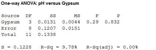
From the ANOVA table, the P-value is 0.832 and the F-value is 0.29.
Decision:
If
If
Since, the level of significance is not specified; the prior level of significance
Conclusion:
Here, the P-value is greater than the level of significance.
That is,
By rejection rule, fails to reject the null hypothesis.
There is sufficient evidence to conclude that the mean pH level differs for the different amounts of gypsum added at
Want to see more full solutions like this?
Chapter 9 Solutions
Statistics for Engineers and Scientists
Additional Math Textbook Solutions
Elementary Statistics ( 3rd International Edition ) Isbn:9781260092561
Elementary Algebra For College Students (10th Edition)
Probability And Statistical Inference (10th Edition)
APPLIED STAT.IN BUS.+ECONOMICS
A First Course in Probability (10th Edition)


- Examine the Variables: Carefully review and note the names of all variables in the dataset. Examples of these variables include: Mileage (mpg) Number of Cylinders (cyl) Displacement (disp) Horsepower (hp) Research: Google to understand these variables. Statistical Analysis: Select mpg variable, and perform the following statistical tests. Once you are done with these tests using mpg variable, repeat the same with hp Mean Median First Quartile (Q1) Second Quartile (Q2) Third Quartile (Q3) Fourth Quartile (Q4) 10th Percentile 70th Percentile Skewness Kurtosis Document Your Results: In RStudio: Before running each statistical test, provide a heading in the format shown at the bottom. “# Mean of mileage – Your name’s command” In Microsoft Word: Once you've completed all tests, take a screenshot of your results in RStudio and paste it into a Microsoft Word document. Make sure that snapshots are very clear. You will need multiple snapshots. Also transfer these results to the…arrow_forward2 (VaR and ES) Suppose X1 are independent. Prove that ~ Unif[-0.5, 0.5] and X2 VaRa (X1X2) < VaRa(X1) + VaRa (X2). ~ Unif[-0.5, 0.5]arrow_forward8 (Correlation and Diversification) Assume we have two stocks, A and B, show that a particular combination of the two stocks produce a risk-free portfolio when the correlation between the return of A and B is -1.arrow_forward
- 9 (Portfolio allocation) Suppose R₁ and R2 are returns of 2 assets and with expected return and variance respectively r₁ and 72 and variance-covariance σ2, 0%½ and σ12. Find −∞ ≤ w ≤ ∞ such that the portfolio wR₁ + (1 - w) R₂ has the smallest risk.arrow_forward7 (Multivariate random variable) Suppose X, €1, €2, €3 are IID N(0, 1) and Y2 Y₁ = 0.2 0.8X + €1, Y₂ = 0.3 +0.7X+ €2, Y3 = 0.2 + 0.9X + €3. = (In models like this, X is called the common factors of Y₁, Y₂, Y3.) Y = (Y1, Y2, Y3). (a) Find E(Y) and cov(Y). (b) What can you observe from cov(Y). Writearrow_forward1 (VaR and ES) Suppose X ~ f(x) with 1+x, if 0> x > −1 f(x) = 1−x if 1 x > 0 Find VaRo.05 (X) and ES0.05 (X).arrow_forward
- Joy is making Christmas gifts. She has 6 1/12 feet of yarn and will need 4 1/4 to complete our project. How much yarn will she have left over compute this solution in two different ways arrow_forwardSolve for X. Explain each step. 2^2x • 2^-4=8arrow_forwardOne hundred people were surveyed, and one question pertained to their educational background. The results of this question and their genders are given in the following table. Female (F) Male (F′) Total College degree (D) 30 20 50 No college degree (D′) 30 20 50 Total 60 40 100 If a person is selected at random from those surveyed, find the probability of each of the following events.1. The person is female or has a college degree. Answer: equation editor Equation Editor 2. The person is male or does not have a college degree. Answer: equation editor Equation Editor 3. The person is female or does not have a college degree.arrow_forward
 MATLAB: An Introduction with ApplicationsStatisticsISBN:9781119256830Author:Amos GilatPublisher:John Wiley & Sons Inc
 Probability and Statistics for Engineering and th...StatisticsISBN:9781305251809Author:Jay L. DevorePublisher:Cengage Learning
 Statistics for The Behavioral Sciences (MindTap C...StatisticsISBN:9781305504912Author:Frederick J Gravetter, Larry B. WallnauPublisher:Cengage Learning
 Elementary Statistics: Picturing the World (7th E...StatisticsISBN:9780134683416Author:Ron Larson, Betsy FarberPublisher:PEARSON
 The Basic Practice of StatisticsStatisticsISBN:9781319042578Author:David S. Moore, William I. Notz, Michael A. FlignerPublisher:W. H. Freeman
 Introduction to the Practice of StatisticsStatisticsISBN:9781319013387Author:David S. Moore, George P. McCabe, Bruce A. CraigPublisher:W. H. Freeman