
Videos
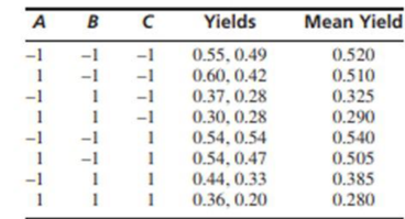
The article “Efficient Pyruvate Production by a Multi-Vitamin Auxotroph of Torulopsis glabrata: Key Role and Optimization of Vitamin Levels” (Y. Li. J. Chen, ct al. Applied Microbiology and Biotechnology, 200l:680–685) investigates the effects of the levels of several vitamins in a cell culture on the yield (in g/L) of pyruvate, a useful organic acid. The data in the following table are presented as two replicates of a 23 design. The factors are A: nicotinic acid. B: thiamine, and C: biotin. (Two statistically insignificant factors have been dropped. In the article, each factor was tested at four levels: we have collapsed these to two.)
- a. Compute estimates of the main effects and interactions, and the sum of squares and P-value for each.
- b. Is the additive model appropriate?
- c. What conclusions about the factors can be drawn from these results?
a.
Obtain the estimates of the main effects and interaction, and sum of squares and P- value for the each treatment combination.
Answer to Problem 4E
The estimates of the main effects and interaction, and sum of squares and P- value for the each treatment combination are given below:
ANOVA table:
| Variable | Effect | DF | Sum of squares | Mean Square | F | P |
| A | –0.04625 | 1 | 0.008556 | 0.008556 | 1.57 | 0.245 |
| B | –0.19875 | 1 | 0.158006 | 0.158006 | 29.03 | 0.001 |
| C | 0.01625 | 1 | 0.001056 | 0.001056 | 0.19 | 0.671 |
| AB | –0.02375 | 1 | 0.002256 | 0.002256 | 0.41 | 0.538 |
| AC | –0.02375 | 1 | 0.002256 | 0.002256 | 0.41 | 0.538 |
| BC | 0.00875 | 1 | 0.000306 | 0.000306 | 0.06 | 0.818 |
| ABC | –0.01125 | 1 | 0.000506 | 0.000506 | 0.09 | 0.768 |
| Error | 8 | 0.043550 | 0.005444 | |||
| Total | 15 |
Explanation of Solution
Given info:
The information is based on conducting the experiment on cell culture on the yield of pyruvate which has two levels for the factors of nicotinic acid (A), thiamine (B), and biotin (C). The experiment of chemical reaction has been conducted twice.
Calculation:
Denote the average yield of the factor A as
Factor A denotes the nicotinic, Factor B denotes the thiamine and Factor C denotes the biotin.
The effect estimate of the treatments is:
The effect estimate of treatment A is:
Substitute the corresponding values of mean yield,
The effect estimate of treatment B is:
The effect estimate of treatment C is:
The effect estimate of treatment AB is:
The effect estimate of treatment AC is:
The effect estimate of treatment BC is:
The effect estimate of treatment ABC is:
The estimates of the main effects and interaction, and sum of squares and P- value for the each treatment combination are given below:
Step-by-step procedure for finding the factorial design table is as follows:
Software procedure:
- Choose Stat > DOE > Factorial > Create Factorial Design.
- Under Type of Design, choose General full factorial design.
- From Number of factors, choose 3.
- Click Designs.
- In Factor A, type A under Name and type 2 Under Number of Levels.
- In Factor B, type B under Name and type 2 Under Number of Levels.
- . In Factor C, type C under Name and type 2 Under Number of Levels.
- From Number of replicates, choose 2.
- Click OK.
- Select Summary table under Results.
- Click OK.
- Enter the corresponding Yield in the newly created factorial design worksheet based on the levels of each factor.
Step-by-step procedure for finding the ANOVA table is as follows:
- Choose Stat > DOE > Factorial > Analyze Factorial Design.
- In Response, enter Yield.
- In Terms, select all the terms.
- In Results, choose “Model summary and ANOVA table”.
- Click OK in all the dialog boxes.
Output obtained by MINITAB procedure is as follows:
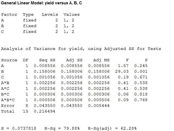
The sum of squares and P- values has been obtained for each treatment combination by using MINITAB.
Thus, the estimates of the main effects and interaction, and sum of squares and P- value for the each treatment combination are given below:
ANOVA table:
| Variable | Effect | DF | Sum of squares | Mean Square | F | P |
| A | –0.04625 | 1 | 0.008556 | 0.008556 | 1.57 | 0.245 |
| B | –0.19875 | 1 | 0.158006 | 0.158006 | 29.03 | 0.001 |
| C | 0.01625 | 1 | 0.001056 | 0.001056 | 0.19 | 0.671 |
| AB | –0.02375 | 1 | 0.002256 | 0.002256 | 0.41 | 0.538 |
| AC | –0.02375 | 1 | 0.002256 | 0.002256 | 0.41 | 0.538 |
| BC | 0.00875 | 1 | 0.000306 | 0.000306 | 0.06 | 0.818 |
| ABC | –0.01125 | 1 | 0.000506 | 0.000506 | 0.09 | 0.768 |
| Error | 8 | 0.043550 | 0.005444 | |||
| Total | 15 |
b.
Check whether the additive model is appropriate.
Answer to Problem 4E
Yes, the additive model is appropriate .
Explanation of Solution
Justification:
Principle rule to hold an additive model:
The additive model is acceptable when the interactions are small.
Hence the additive model is appropriate but interaction effect obtained in previous part (a) does not provide significant results.
c.
State whether any main effects and interaction are important.
Answer to Problem 4E
There is sufficient evidence to conclude that there is no significant difference between the means of two levels in main effect A at
There is sufficient evidence to conclude that there is significant difference between the means of two levels in main effect B at
There is sufficient evidence to conclude that there is no significant difference between the means of two levels in main effect C at
There is sufficient evidence to conclude that the interaction is not significant at
Explanation of Solution
Calculation:
The testing of hypotheses is as follows:
State the hypotheses:
Main factor A:
Null hypothesis:
Alternative hypothesis:
Main factor B:
Null hypothesis:
Alternative hypothesis:
Interaction AB:
Null hypothesis:
Alternative hypothesis:
Interaction AC:
Null hypothesis:
Alternative hypothesis:
Interaction BC:
Null hypothesis:
Alternative hypothesis:
Interaction ABC:
Null hypothesis:
Alternative hypothesis:
Assume that the level of significance as 0.05.
From the MINITAB output obtained in previous part (a), the P- value for main effects and interaction are given below:
| Treatment | P |
| A | 0.245 |
| B | 0.001 |
| C | 0.671 |
| AB | 0.538 |
| AC | 0.538 |
| BC | 0.818 |
| ABC | 0.768 |
Decision:
If
If
Conclusion:
Factor A:
Here, the P-value is greater than the level of significance.
That is,
By rejection rule, fail to reject the null hypothesis.
Thus, there is sufficient evidence to conclude that there is no significant difference between the means of two levels in main effect A at
Factor B:
Here, the P-value is less than the level of significance.
That is,
By rejection rule, reject the null hypothesis.
Thus, there is sufficient evidence to conclude that there is significant difference between the means of two levels in main effect B at
Factor C:
Here, the P-value is greater than the level of significance.
That is,
By rejection rule, fail to reject the null hypothesis.
Thus, there is sufficient evidence to conclude that there is no significant difference between the means of two levels in main effect C at
Interaction AB:
Here, the P-value is greater than the level of significance.
That is,
By rejection rule, fail to reject the null hypothesis.
Thus, there is sufficient evidence to conclude that the interaction AB is not significant at
Interaction AC:
Here, the P-value is greater than the level of significance.
That is,
By rejection rule, fail to reject the null hypothesis.
Thus, there is sufficient evidence to conclude that the interaction AC is not significant at
Interaction BC:
Here, the P-value is greater than the level of significance.
That is,
By rejection rule, fail to reject the null hypothesis.
Thus, there is sufficient evidence to conclude that the interaction BC is not significant at
Interaction ABC:
Here, the P-value is greater than the level of significance.
That is,
By rejection rule, fail to reject the null hypothesis.
Thus, there is sufficient evidence to conclude that the interaction ABC is not significant at
Hence the P-value of Factor B states that it has more effect on the yield than Factor A and Factor C.
Want to see more full solutions like this?
Chapter 9 Solutions
Statistics for Engineers and Scientists
Additional Math Textbook Solutions
APPLIED STAT.IN BUS.+ECONOMICS
Calculus: Early Transcendentals (2nd Edition)
Mathematics for the Trades: A Guided Approach (11th Edition) (What's New in Trade Math)
Elementary Statistics: Picturing the World (7th Edition)
A Problem Solving Approach To Mathematics For Elementary School Teachers (13th Edition)


- Techniques QUAT6221 2025 PT B... TM Tabudi Maphoru Activities Assessments Class Progress lIE Library • Help v The table below shows the prices (R) and quantities (kg) of rice, meat and potatoes items bought during 2013 and 2014: 2013 2014 P1Qo PoQo Q1Po P1Q1 Price Ро Quantity Qo Price P1 Quantity Q1 Rice 7 80 6 70 480 560 490 420 Meat 30 50 35 60 1 750 1 500 1 800 2 100 Potatoes 3 100 3 100 300 300 300 300 TOTAL 40 230 44 230 2 530 2 360 2 590 2 820 Instructions: 1 Corall dawn to tha bottom of thir ceraan urina se se tha haca nariad in archerca antarand cubmit Q Search ENG US 口X 2025/05arrow_forwardThe table below indicates the number of years of experience of a sample of employees who work on a particular production line and the corresponding number of units of a good that each employee produced last month. Years of Experience (x) Number of Goods (y) 11 63 5 57 1 48 4 54 45 3 51 Q.1.1 By completing the table below and then applying the relevant formulae, determine the line of best fit for this bivariate data set. Do NOT change the units for the variables. X y X2 xy Ex= Ey= EX2 EXY= Q.1.2 Estimate the number of units of the good that would have been produced last month by an employee with 8 years of experience. Q.1.3 Using your calculator, determine the coefficient of correlation for the data set. Interpret your answer. Q.1.4 Compute the coefficient of determination for the data set. Interpret your answer.arrow_forwardQ.3.2 A sample of consumers was asked to name their favourite fruit. The results regarding the popularity of the different fruits are given in the following table. Type of Fruit Number of Consumers Banana 25 Apple 20 Orange 5 TOTAL 50 Draw a bar chart to graphically illustrate the results given in the table.arrow_forward
- Q.2.3 The probability that a randomly selected employee of Company Z is female is 0.75. The probability that an employee of the same company works in the Production department, given that the employee is female, is 0.25. What is the probability that a randomly selected employee of the company will be female and will work in the Production department? Q.2.4 There are twelve (12) teams participating in a pub quiz. What is the probability of correctly predicting the top three teams at the end of the competition, in the correct order? Give your final answer as a fraction in its simplest form.arrow_forwardQ.2.1 A bag contains 13 red and 9 green marbles. You are asked to select two (2) marbles from the bag. The first marble selected will not be placed back into the bag. Q.2.1.1 Construct a probability tree to indicate the various possible outcomes and their probabilities (as fractions). Q.2.1.2 What is the probability that the two selected marbles will be the same colour? Q.2.2 The following contingency table gives the results of a sample survey of South African male and female respondents with regard to their preferred brand of sports watch: PREFERRED BRAND OF SPORTS WATCH Samsung Apple Garmin TOTAL No. of Females 30 100 40 170 No. of Males 75 125 80 280 TOTAL 105 225 120 450 Q.2.2.1 What is the probability of randomly selecting a respondent from the sample who prefers Garmin? Q.2.2.2 What is the probability of randomly selecting a respondent from the sample who is not female? Q.2.2.3 What is the probability of randomly…arrow_forwardTest the claim that a student's pulse rate is different when taking a quiz than attending a regular class. The mean pulse rate difference is 2.7 with 10 students. Use a significance level of 0.005. Pulse rate difference(Quiz - Lecture) 2 -1 5 -8 1 20 15 -4 9 -12arrow_forward
- The following ordered data list shows the data speeds for cell phones used by a telephone company at an airport: A. Calculate the Measures of Central Tendency from the ungrouped data list. B. Group the data in an appropriate frequency table. C. Calculate the Measures of Central Tendency using the table in point B. D. Are there differences in the measurements obtained in A and C? Why (give at least one justified reason)? I leave the answers to A and B to resolve the remaining two. 0.8 1.4 1.8 1.9 3.2 3.6 4.5 4.5 4.6 6.2 6.5 7.7 7.9 9.9 10.2 10.3 10.9 11.1 11.1 11.6 11.8 12.0 13.1 13.5 13.7 14.1 14.2 14.7 15.0 15.1 15.5 15.8 16.0 17.5 18.2 20.2 21.1 21.5 22.2 22.4 23.1 24.5 25.7 28.5 34.6 38.5 43.0 55.6 71.3 77.8 A. Measures of Central Tendency We are to calculate: Mean, Median, Mode The data (already ordered) is: 0.8, 1.4, 1.8, 1.9, 3.2, 3.6, 4.5, 4.5, 4.6, 6.2, 6.5, 7.7, 7.9, 9.9, 10.2, 10.3, 10.9, 11.1, 11.1, 11.6, 11.8, 12.0, 13.1, 13.5, 13.7, 14.1, 14.2, 14.7, 15.0, 15.1, 15.5,…arrow_forwardPEER REPLY 1: Choose a classmate's Main Post. 1. Indicate a range of values for the independent variable (x) that is reasonable based on the data provided. 2. Explain what the predicted range of dependent values should be based on the range of independent values.arrow_forwardIn a company with 80 employees, 60 earn $10.00 per hour and 20 earn $13.00 per hour. Is this average hourly wage considered representative?arrow_forward
- The following is a list of questions answered correctly on an exam. Calculate the Measures of Central Tendency from the ungrouped data list. NUMBER OF QUESTIONS ANSWERED CORRECTLY ON AN APTITUDE EXAM 112 72 69 97 107 73 92 76 86 73 126 128 118 127 124 82 104 132 134 83 92 108 96 100 92 115 76 91 102 81 95 141 81 80 106 84 119 113 98 75 68 98 115 106 95 100 85 94 106 119arrow_forwardThe following ordered data list shows the data speeds for cell phones used by a telephone company at an airport: A. Calculate the Measures of Central Tendency using the table in point B. B. Are there differences in the measurements obtained in A and C? Why (give at least one justified reason)? 0.8 1.4 1.8 1.9 3.2 3.6 4.5 4.5 4.6 6.2 6.5 7.7 7.9 9.9 10.2 10.3 10.9 11.1 11.1 11.6 11.8 12.0 13.1 13.5 13.7 14.1 14.2 14.7 15.0 15.1 15.5 15.8 16.0 17.5 18.2 20.2 21.1 21.5 22.2 22.4 23.1 24.5 25.7 28.5 34.6 38.5 43.0 55.6 71.3 77.8arrow_forwardIn a company with 80 employees, 60 earn $10.00 per hour and 20 earn $13.00 per hour. a) Determine the average hourly wage. b) In part a), is the same answer obtained if the 60 employees have an average wage of $10.00 per hour? Prove your answer.arrow_forward
 MATLAB: An Introduction with ApplicationsStatisticsISBN:9781119256830Author:Amos GilatPublisher:John Wiley & Sons Inc
 Probability and Statistics for Engineering and th...StatisticsISBN:9781305251809Author:Jay L. DevorePublisher:Cengage Learning
 Statistics for The Behavioral Sciences (MindTap C...StatisticsISBN:9781305504912Author:Frederick J Gravetter, Larry B. WallnauPublisher:Cengage Learning
 Elementary Statistics: Picturing the World (7th E...StatisticsISBN:9780134683416Author:Ron Larson, Betsy FarberPublisher:PEARSON
 The Basic Practice of StatisticsStatisticsISBN:9781319042578Author:David S. Moore, William I. Notz, Michael A. FlignerPublisher:W. H. Freeman
 Introduction to the Practice of StatisticsStatisticsISBN:9781319013387Author:David S. Moore, George P. McCabe, Bruce A. CraigPublisher:W. H. Freeman