
Repeat Prob. 8.45, but incorporate the fact that the friction factor can be computed with the von Karman equation,
where
where
To calculate: The flow in every pipe length shown in Fig. P8.45 by writing a program in a mathematics software package, if the friction factor can be computed with the von Karman equation,
Answer to Problem 46P
Solution:
Therefore, the flows in each pipe length in
Explanation of Solution
Given Information:
Refer to Figure P8.45.
Refer to the problem 8.45.
A fluid is pumped into the network of pipes shown in Fig. P8.45. At steady state, the following flow balances must hold,
Here,
Pipe lengths are either
Write the von Karman equation,
Where, Re is the Reynolds Number. The formula to calculate Re is shown below,
Where,
For circular pipes V is obtained as following,
The viscosity of the fluid is
Formula Used:
Write the expression for the pressure drop.
Here,
For circular pipes V is obtained as following,
Calculation:
The Pipe sectional flow is available only for pipe 1 thus, to calculate the velocity of the fluid in the all pipe use sectional flow data which will help in calculating the Reynolds Number and in turn the friction factor from the Von-Karman Equation.
Here 10 different friction factor values will be available thus, the need necessary changes to the pressure calculation.
Use the Bisection Algorithm in MATLAB to decode the Von-Karman Equation and find out the root.
Hence unlike the previous sum where friction factor was constant; here 10 different friction factor values will be available and the necessary changes need to be incorporated in the pressure calculation.
Use the Bisection Algorithm in MATLAB to decode the Von-Karman Equation and find out the root.
Consider the following MATLAB code for the Bisection Algorithm,
while
if(
break;
elseif(
else
end
end
Solve for Pipe 1,
Consider the following formula for V,
Substitute the values,
Consider the following formula for Reynolds Number,
Substitute the values,
Hence,
Consider the following MATLAB session to obtain the output,
Hence:
Solve for Pipe 2,
Consider the following formula for V,
Substitute the values,
Consider the following formula for Reynolds Number,
Substitute the values,
Hence,
Consider the following MATLAB session to obtain the output,
Hence:
For Pipe 3:
Consider the following formula for V,
Substitute the values,
Consider the following formula for Reynolds Number,
Substitute the values,
Hence, Re =110039.
Consider the following MATLAB session to obtain the output,
Hence:
For Pipe 4:
Consider the following formula for V,
Substitute the values,
Consider the following formula for Reynolds Number,
Substitute the values,
Hence,
Consider the following MATLAB session to obtain the output,
Hence:
For Pipe 5:
Consider the following formula for V,
Substitute the values,
Consider the following formula for Reynolds Number,
Substitute the values,
Hence,
Consider the following MATLAB session to obtain the output,
Hence:
For Pipe 6:
Consider the following formula for V,
Substitute the values,
Consider the following formula for Reynolds Number,
Substitute the values,
Hence,
Consider the following MATLAB session to obtain the output,
Hence:
For Pipe 7:
Consider the following formula for V,
Substitute the values,
Consider the following formula for Reynolds Number,
Substitute the values,
Hence
Consider the following MATLAB session to obtain the output,
Hence:
For Pipe 8:
Consider the following formula for V,
Substitute the values,
Consider the following formula for Reynolds Number,
Substitute the values,
Hence
Consider the following MATLAB session to obtain the output,
Hence:
For Pipe 9:
Consider the following formula for V,
Substitute the values,
Consider the following formula for Reynolds Number,
Substitute the values,
Hence,
Consider the following MATLAB session to obtain the output,
Hence:
Now the friction factor will not play any role for section 10 of the pipe because the flow in section 10 of the pipe is depended upon section 2 and section 9.
After calculating the friction factor for different section of the pipe, the Excel will be used to solve the existing Equations.
Starting with Excel Solver,
Step 1:
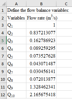
First define the variables that need to be found out: Flow rate
The variable definition is shown below:
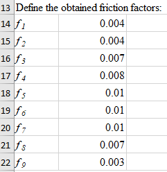
Next define the friction factors:
Step 2:
In each circular pipe length calculate the sectional pressure drop.
Consider the following formula for the pressure drop,
Here
Also,
And
With Q is the flow rate in
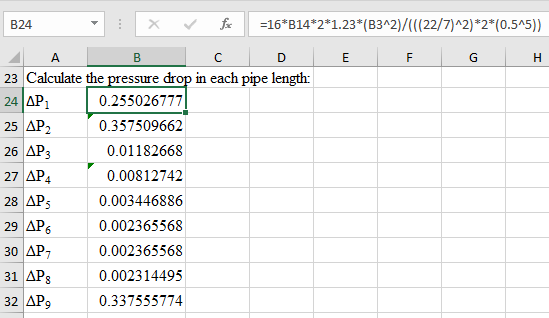
Note: The formula in the formula bar shows the Pressure calculation for
Now the pressure in other section of the pipes are calculated and shown in consequent cells with friction factor of
Step 3:
Constraint Setting:
Following are the required constraints or in other words the Equations to be solved:
And for pressure drops,
Also,
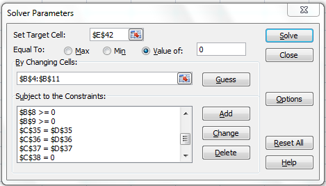
Since there is nothing to maximize or minimize, the pressure drop is the summation of three right hand loops, that is summation of cells: C28+C29+C30 is set to zero. In doing so, not only is the driving condition being set, but also no additional conditions are being added to alter the fate of the equations.
Once the arrangements are made, call Solver as shown below:
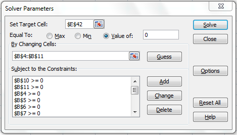
Continued after scroll down is shown below,
Next, click on Solve. The results are displayed below,
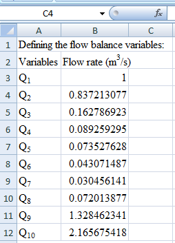
Therefore, the flows in each pipe length in
Want to see more full solutions like this?
Chapter 8 Solutions
Numerical Methods for Engineers
Additional Math Textbook Solutions
Precalculus: A Unit Circle Approach (3rd Edition)
Pathways To Math Literacy (looseleaf)
Elementary Statistics: Picturing the World (7th Edition)
Precalculus
Elementary & Intermediate Algebra
Precalculus: Mathematics for Calculus (Standalone Book)
- y = log 5 – x2 - 4 00arrow_forwardPlease fill in the rest of the steps of the proof of Thm 2.5. Show how "Repeating this step with n-1,n-2,...,2 in place of n" gives us the desired result.arrow_forwardConsider the initial value problem y"+y'-12y= 0, y(0) = a, y'(0) = 4 Find the value of a so that the solution to the initial value problem approaches zero as too a =arrow_forward
- No ai Plz All partsarrow_forwardNo chatgpt pls will upvote Already got wrong chatgpt answerarrow_forwardYour employer automatically puts 5 percent of your salary into a 401(k) retirement account each year. The account earns 10% interest. Suppose you just got the job, your starting salary is $60000, and you expect to receive a 2.5% raise each year. For simplicity, assume that interest earned and your raises are given as nominal rates and compound continuously. Find the value of your retirement account after 20 yearsarrow_forward
- Compute the principal values of i¹² (i — 1)² and (i(i − 1))². - -arrow_forward1 2 3 Consider the matrix A = 0 4 5. Give an example of 006 (a) a nonzero matrix B for which det(A + B) = det(A) + det(B); (b) a matrix C for which det(A+C)det(A) + det(C).arrow_forwardFind all points at which f(z) = y² sin x + iy is analytic.arrow_forward
 College Algebra (MindTap Course List)AlgebraISBN:9781305652231Author:R. David Gustafson, Jeff HughesPublisher:Cengage Learning
 Trigonometry (MindTap Course List)TrigonometryISBN:9781337278461Author:Ron LarsonPublisher:Cengage Learning
 Linear Algebra: A Modern IntroductionAlgebraISBN:9781285463247Author:David PoolePublisher:Cengage Learning


