
a.
To calculate: The linear regression equation for the population of Hawaii.
The obtained matrix is
Given Information:
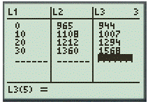
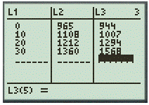
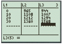
The table is defined,
| Time (years) | Hawaii (thousands) | Idaho (thousands) |
| 1980 | 965 | 944 |
| 1990 | 1108 | 1007 |
| 2000 | 1212 | 1294 |
| 2010 | 1360 | 1568 |
Calculation:
Consider the given table,
| Time (years) | Hawaii (thousands) | Idaho (thousands) |
| 1980 | 965 | 944 |
| 1990 | 1108 | 1007 |
| 2000 | 1212 | 1294 |
| 2010 | 1360 | 1568 |
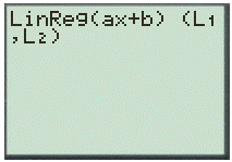
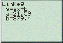
Use a graphing calculator to find the linear rgeression.
Step 1. Insert the table in calculator by using the table feature.
Step 2. Use the LinReg feature with first two list
And,
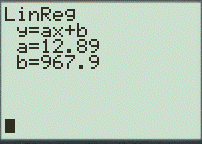
Therefore, the obtained equation is
b.
To calculate: The linear regression equation for the population of Ladho.
The obtained model is
Given Information:
The table is defined,
| Time (years) | Hawaii (thousands) | Ldaho (thousands) |
| 1980 | 965 | 944 |
| 1990 | 1108 | 1007 |
| 2000 | 1212 | 1294 |
| 2010 | 1360 | 1568 |
Calculation:
Consider the given table,
| Time (years) | Hawaii (thousands) | Ldaho (thousands) |
| 1980 | 965 | 944 |
| 1990 | 1108 | 1007 |
| 2000 | 1212 | 1294 |
| 2010 | 1360 | 1568 |
Use a graphing calculator to find the logestic model.
Step 1. Insert the table in calculator by using the table feature.
Step 2. Use the LinReg feature with first two list
Hence, the obtained result is
c.
To Graph: The models in parts (a) and (b) and use these models to explain when the populations of the two states were about the same.
The obtained graph is defined as,
Given Information:
The table is defined,
| Time (years) | Hawaii (thousands) | Ldaho (thousands) |
| 1980 | 965 | 944 |
| 1990 | 1108 | 1007 |
| 2000 | 1212 | 1294 |
| 2010 | 1360 | 1568 |
Calculation:
Consider the given table,
| Time (years) | Hawaii (thousands) | Ldaho (thousands) |
| 1980 | 965 | 944 |
| 1990 | 1108 | 1007 |
| 2000 | 1212 | 1294 |
| 2010 | 1360 | 1568 |
Use a graphing calculator to find the logestic model.
Step 1. Insert the table in calculator by using the table feature.
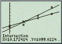
Step 2. Graph the both equations (a) and (b) then use the intersect feature to find the intersection point.
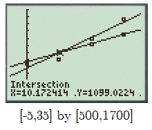
The x -coordinates of the point of intersection is 10.2, and it is representing year 1990.
Hence, the obtained years is 1990.
d.
To determine: The models, which appears to be a better fit for the data and explain which model would you choose to make predictions beyond 2020
Hawaii is having a linear model and Idaho population is having exponential or logistic
Given Information:
The table is defined,
| Time (years) | Hawaii (thousands) | Ldaho (thousands) |
| 1980 | 965 | 944 |
| 1990 | 1108 | 1007 |
| 2000 | 1212 | 1294 |
| 2010 | 1360 | 1568 |
Calculation:
Consider the given information,
The linear model seems to be a good fit for Hawaii as most points appear to be on the line which means that there is almost a constant change in population.
An exponential or a logistic model seems to be appropriate for Idaho since there is a sudden increase in population for the same year intervals which is from 1990 to 2000.
Hence, Hawaii is having a linear model and Idaho population is having exponential or logistic
Chapter 7 Solutions
PRECALCULUS:GRAPHICAL,...-NASTA ED.

- Consider the function f(x) = x²-1. (a) Find the instantaneous rate of change of f(x) at x=1 using the definition of the derivative. Show all your steps clearly. (b) Sketch the graph of f(x) around x = 1. Draw the secant line passing through the points on the graph where x 1 and x-> 1+h (for a small positive value of h, illustrate conceptually). Then, draw the tangent line to the graph at x=1. Explain how the slope of the tangent line relates to the value you found in part (a). (c) In a few sentences, explain what the instantaneous rate of change of f(x) at x = 1 represents in the context of the graph of f(x). How does the rate of change of this function vary at different points?arrow_forward1. The graph of ƒ is given. Use the graph to evaluate each of the following values. If a value does not exist, state that fact. и (a) f'(-5) (b) f'(-3) (c) f'(0) (d) f'(5) 2. Find an equation of the tangent line to the graph of y = g(x) at x = 5 if g(5) = −3 and g'(5) = 4. - 3. If an equation of the tangent line to the graph of y = f(x) at the point where x 2 is y = 4x — 5, find ƒ(2) and f'(2).arrow_forwardDoes the series converge or divergearrow_forward
- Suppose that a particle moves along a straight line with velocity v (t) = 62t, where 0 < t <3 (v(t) in meters per second, t in seconds). Find the displacement d (t) at time t and the displacement up to t = 3. d(t) ds = ["v (s) da = { The displacement up to t = 3 is d(3)- meters.arrow_forwardLet f (x) = x², a 3, and b = = 4. Answer exactly. a. Find the average value fave of f between a and b. fave b. Find a point c where f (c) = fave. Enter only one of the possible values for c. c=arrow_forwardplease do Q3arrow_forward
- Use the properties of logarithms, given that In(2) = 0.6931 and In(3) = 1.0986, to approximate the logarithm. Use a calculator to confirm your approximations. (Round your answers to four decimal places.) (a) In(0.75) (b) In(24) (c) In(18) 1 (d) In ≈ 2 72arrow_forwardFind the indefinite integral. (Remember the constant of integration.) √tan(8x) tan(8x) sec²(8x) dxarrow_forwardFind the indefinite integral by making a change of variables. (Remember the constant of integration.) √(x+4) 4)√6-x dxarrow_forward
 Calculus: Early TranscendentalsCalculusISBN:9781285741550Author:James StewartPublisher:Cengage Learning
 Thomas' Calculus (14th Edition)CalculusISBN:9780134438986Author:Joel R. Hass, Christopher E. Heil, Maurice D. WeirPublisher:PEARSON
 Calculus: Early Transcendentals (3rd Edition)CalculusISBN:9780134763644Author:William L. Briggs, Lyle Cochran, Bernard Gillett, Eric SchulzPublisher:PEARSON
 Calculus: Early TranscendentalsCalculusISBN:9781319050740Author:Jon Rogawski, Colin Adams, Robert FranzosaPublisher:W. H. Freeman
 Calculus: Early Transcendental FunctionsCalculusISBN:9781337552516Author:Ron Larson, Bruce H. EdwardsPublisher:Cengage Learning