Concept explainers
Videos
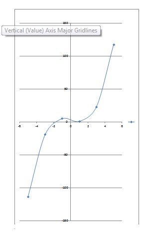
Approximate the solution(s) to using a graphing utility. (pp. 26-28)
To find: Approximate the solution(s) to using a graphing utility.
Answer to Problem 4AYU
The solution is the of the point of intersection .
Explanation of Solution
Given:
Calculation:
The ZERO (or ROOT) feature of a graphing utility can be used to find the solutions of an equation when one side of the equation is 0. In using this feature to solve equations, make use of the fact that when the graph of an equation in two variables, and , crosses or touches the then . For this reason, any value of for which will be a solution to the equation. That is, solving an equation for when one side of the equation is 0 is equivalent to finding where the graph of the corresponding equation in two variables crosses or touches the .
When a graphing utility is used to solve an equation, usually approximate solutions are obtained. Unless otherwise stated, we shall follow the practice of giving approximate solutions as decimals rounded to two decimal places.
Steps for Approximating Solutions of Equations Using ZERO (or ROOT).
Step 1: Write the equation in the form .
Step 2: Graph .
Be sure that the graph is complete. That is, be sure that all the are shown on the screen.
Step 3: Use ZERO (or ROOT) to determine each of the graph.
See on the graph, we can find the intersection of values and solving the graph algebraically.
We get the solution of the of the point of intersection .
Chapter 5 Solutions
Precalculus Enhanced with Graphing Utilities
Additional Math Textbook Solutions
Pre-Algebra Student Edition
Algebra and Trigonometry (6th Edition)
College Algebra with Modeling & Visualization (5th Edition)
Intro Stats, Books a la Carte Edition (5th Edition)
Elementary Statistics: Picturing the World (7th Edition)


- (7) (12 points) Let F(x, y, z) = (y, x+z cos yz, y cos yz). Ꮖ (a) (4 points) Show that V x F = 0. (b) (4 points) Find a potential f for the vector field F. (c) (4 points) Let S be a surface in R3 for which the Stokes' Theorem is valid. Use Stokes' Theorem to calculate the line integral Jos F.ds; as denotes the boundary of S. Explain your answer.arrow_forward(3) (16 points) Consider z = uv, u = x+y, v=x-y. (a) (4 points) Express z in the form z = fog where g: R² R² and f: R² → R. (b) (4 points) Use the chain rule to calculate Vz = (2, 2). Show all intermediate steps otherwise no credit. (c) (4 points) Let S be the surface parametrized by T(x, y) = (x, y, ƒ (g(x, y)) (x, y) = R². Give a parametric description of the tangent plane to S at the point p = T(x, y). (d) (4 points) Calculate the second Taylor polynomial Q(x, y) (i.e. the quadratic approximation) of F = (fog) at a point (a, b). Verify that Q(x,y) F(a+x,b+y). =arrow_forward(6) (8 points) Change the order of integration and evaluate (z +4ry)drdy . So S√ ² 0arrow_forward
- (10) (16 points) Let R>0. Consider the truncated sphere S given as x² + y² + (z = √15R)² = R², z ≥0. where F(x, y, z) = −yi + xj . (a) (8 points) Consider the vector field V (x, y, z) = (▼ × F)(x, y, z) Think of S as a hot-air balloon where the vector field V is the velocity vector field measuring the hot gasses escaping through the porous surface S. The flux of V across S gives the volume flow rate of the gasses through S. Calculate this flux. Hint: Parametrize the boundary OS. Then use Stokes' Theorem. (b) (8 points) Calculate the surface area of the balloon. To calculate the surface area, do the following: Translate the balloon surface S by the vector (-15)k. The translated surface, call it S+ is part of the sphere x² + y²+z² = R². Why do S and S+ have the same area? ⚫ Calculate the area of S+. What is the natural spherical parametrization of S+?arrow_forward(1) (8 points) Let c(t) = (et, et sint, et cost). Reparametrize c as a unit speed curve starting from the point (1,0,1).arrow_forward(9) (16 points) Let F(x, y, z) = (x² + y − 4)i + 3xyj + (2x2 +z²)k = - = (x²+y4,3xy, 2x2 + 2²). (a) (4 points) Calculate the divergence and curl of F. (b) (6 points) Find the flux of V x F across the surface S given by x² + y²+2² = 16, z ≥ 0. (c) (6 points) Find the flux of F across the boundary of the unit cube E = [0,1] × [0,1] x [0,1].arrow_forward
- (8) (12 points) (a) (8 points) Let C be the circle x² + y² = 4. Let F(x, y) = (2y + e²)i + (x + sin(y²))j. Evaluate the line integral JF. F.ds. Hint: First calculate V x F. (b) (4 points) Let S be the surface r² + y² + z² = 4, z ≤0. Calculate the flux integral √(V × F) F).dS. Justify your answer.arrow_forwardDetermine whether the Law of Sines or the Law of Cosines can be used to find another measure of the triangle. a = 13, b = 15, C = 68° Law of Sines Law of Cosines Then solve the triangle. (Round your answers to four decimal places.) C = 15.7449 A = 49.9288 B = 62.0712 × Need Help? Read It Watch Itarrow_forward(4) (10 points) Evaluate √(x² + y² + z²)¹⁄² exp[}(x² + y² + z²)²] dV where D is the region defined by 1< x² + y²+ z² ≤4 and √√3(x² + y²) ≤ z. Note: exp(x² + y²+ 2²)²] means el (x²+ y²+=²)²]¸arrow_forward
- (2) (12 points) Let f(x,y) = x²e¯. (a) (4 points) Calculate Vf. (b) (4 points) Given x directional derivative 0, find the line of vectors u = D₁f(x, y) = 0. (u1, 2) such that the - (c) (4 points) Let u= (1+3√3). Show that Duƒ(1, 0) = ¦|▼ƒ(1,0)| . What is the angle between Vf(1,0) and the vector u? Explain.arrow_forwardFind the missing values by solving the parallelogram shown in the figure. (The lengths of the diagonals are given by c and d. Round your answers to two decimal places.) a b 29 39 66.50 C 17.40 d 0 54.0 126° a Ꮎ b darrow_forward(5) (10 points) Let D be the parallelogram in the xy-plane with vertices (0, 0), (1, 1), (1, 1), (0, -2). Let f(x,y) = xy/2. Use the linear change of variables T(u, v)=(u,u2v) = (x, y) 1 to calculate the integral f(x,y) dA= 0 ↓ The domain of T is a rectangle R. What is R? |ǝ(x, y) du dv. |ð(u, v)|arrow_forward
 Calculus: Early TranscendentalsCalculusISBN:9781285741550Author:James StewartPublisher:Cengage Learning
 Thomas' Calculus (14th Edition)CalculusISBN:9780134438986Author:Joel R. Hass, Christopher E. Heil, Maurice D. WeirPublisher:PEARSON
 Calculus: Early Transcendentals (3rd Edition)CalculusISBN:9780134763644Author:William L. Briggs, Lyle Cochran, Bernard Gillett, Eric SchulzPublisher:PEARSON
 Calculus: Early TranscendentalsCalculusISBN:9781319050740Author:Jon Rogawski, Colin Adams, Robert FranzosaPublisher:W. H. Freeman
 Calculus: Early Transcendental FunctionsCalculusISBN:9781337552516Author:Ron Larson, Bruce H. EdwardsPublisher:Cengage Learning