
Concept explainers
Videos
(a)
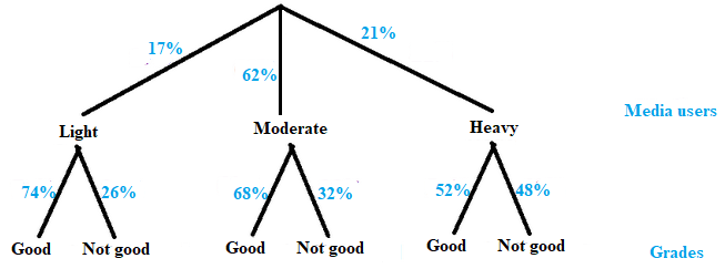
Represent this chance process with Tree diagram.
(a)
Explanation of Solution
Given information:
Study about media influence in young people lives aged 8 − 18:
17% were classified as light media users
62% were classified as moderate media users
21% were classified as heavy media users
Respondents with good grades:
74% light users described their grades as good
68% moderate users described their grades as good
52% heavy users described their grades as good
First level:
First level consists of three types of media users:
Light, moderate and heavy
Thus,
The first level requires three children:
Light, moderate and heavy
Second level:
In this level, there are two types of grades:
Good grades or No Good grades
Thus,
The second level consists of two children per child at the first level i.e.; Good grades or No Good grades.
The required tree diagram can be drawn as:
(b)
(b)
Answer to Problem 82E
Probability for the person with good grades is 0.6566.
Explanation of Solution
Given information:
Study about media influence in young people lives aged 8 − 18:
17% were classified as light media users
62% were classified as moderate media users
21% were classified as heavy media users
Respondents with good grades:
74% light users described their grades as good
68% moderate users described their grades as good
52% heavy users described their grades as good
Calculations:
According to the general multiplication rule,
According to the
Let
L: Light user
M: Moderate user
H: Heavy user
G: Good grades
Gc: No Good grades
Now,
The corresponding probabilities:
Probability for light user,
Probability for moderate user,
Probability for heavy user,
Probability for light user with good grades,
Probability for moderate user with good grades,
Probability for heavy user with good grades,
Apply general multiplication rule:
Probability for user with good grades and light user,
Probability for user with good grades and moderate user,
Probability for user with good grades and heavy user,
Since each person cannot become more than one type of user.
Apply the addition rule for mutually exclusive events:
Thus,
Probability for the person describes his or her grades as good is 0.6566.
(c)
Conditional probability for the randomly chosen person describes his or her grade as good is a heavy user of media.
(c)
Answer to Problem 82E
Probability that the randomly chosen person describes his or her grade as good is a heavy user of media is approx. 0.1663.
Explanation of Solution
Given information:
Study about media influence in young people lives aged 8 − 18:
17% were classified as light media users
62% were classified as moderate media users
21% were classified as heavy media users
Respondents with good grades:
74% light users described their grades as good
68% moderate users described their grades as good
52% heavy users described their grades as good
Calculations:
According to the conditional probability,
From Part (b),
We have
Probability for the person describes his or her grades as good,
Probability for user with good grades and heavy user,
Apply the conditional probability:
Thus,
The probability for the person describes his or her grades as good is a heavy user of media is approx. 0.1663.
Chapter 5 Solutions
PRACTICE OF STATISTICS F/AP EXAM
Additional Math Textbook Solutions
Thinking Mathematically (6th Edition)
Basic Business Statistics, Student Value Edition
University Calculus: Early Transcendentals (4th Edition)
Elementary Statistics
A Problem Solving Approach To Mathematics For Elementary School Teachers (13th Edition)
A First Course in Probability (10th Edition)


- A marketing agency wants to determine whether different advertising platforms generate significantly different levels of customer engagement. The agency measures the average number of daily clicks on ads for three platforms: Social Media, Search Engines, and Email Campaigns. The agency collects data on daily clicks for each platform over a 10-day period and wants to test whether there is a statistically significant difference in the mean number of daily clicks among these platforms. Conduct ANOVA test. You can provide your answer by inserting a text box and the answer must include: also please provide a step by on getting the answers in excel Null hypothesis, Alternative hypothesis, Show answer (output table/summary table), and Conclusion based on the P value.arrow_forwardA company found that the daily sales revenue of its flagship product follows a normal distribution with a mean of $4500 and a standard deviation of $450. The company defines a "high-sales day" that is, any day with sales exceeding $4800. please provide a step by step on how to get the answers Q: What percentage of days can the company expect to have "high-sales days" or sales greater than $4800? Q: What is the sales revenue threshold for the bottom 10% of days? (please note that 10% refers to the probability/area under bell curve towards the lower tail of bell curve) Provide answers in the yellow cellsarrow_forwardBusiness Discussarrow_forward
 MATLAB: An Introduction with ApplicationsStatisticsISBN:9781119256830Author:Amos GilatPublisher:John Wiley & Sons Inc
 Probability and Statistics for Engineering and th...StatisticsISBN:9781305251809Author:Jay L. DevorePublisher:Cengage Learning
 Statistics for The Behavioral Sciences (MindTap C...StatisticsISBN:9781305504912Author:Frederick J Gravetter, Larry B. WallnauPublisher:Cengage Learning
 Elementary Statistics: Picturing the World (7th E...StatisticsISBN:9780134683416Author:Ron Larson, Betsy FarberPublisher:PEARSON
 The Basic Practice of StatisticsStatisticsISBN:9781319042578Author:David S. Moore, William I. Notz, Michael A. FlignerPublisher:W. H. Freeman
 Introduction to the Practice of StatisticsStatisticsISBN:9781319013387Author:David S. Moore, George P. McCabe, Bruce A. CraigPublisher:W. H. Freeman